This project involves capturing images of an object from multiple view points and building a 3D model out of it. This model will be further used to perform image based rendering of the object from novel viewpoints.

The project augments the initial phase of Biswarup's PhD work. The currently available system has been tested on synthetic inputs from rendered 3D scenes. The main goal of my project will be to build an image acquisition system which will simplify the process of capturing images of real-world objects.

My goal in this phase was to verify if the existing system indeed works on real data. To do this, I familiarised myself with the existing codebase and user interface. I reworked the datasets from a previous 3D reconstruction project and tested if the resulting 3D models were convincing. Certain assumptions of the original codebase were no longer valid and were rectified. The most major of these was the assumption that images are taken by moving the camera on the surface of a sphere of fixed radius around the object. This was modified to allow arbitrary distance between object and camera. Here are the results of this test:

This stage involved setting up an acquisition system for taking images of an object from various viewpoints. It was decided that we would require a mechanised turn table to make the object rotate at regular intervals of time. This turntable has been procured from the SPANN lab of the Electrical Dept.

A camera is mounted on a tripod at a fixed height and distance from the table. The table and the background are covered with a uniform coloured diffuse surface (sheets of paper). Ambient lighting is achieved by using flood lights reflected off thermocol sheets from behind the camera. This ensures that most of the shadows are behind the object and do not show up in the captured images.

A complication that occurs due to the light source behind the camera is that the camera and tripod now cast diffused shadows on the table surface. To prevent this from causing any problems, a set of basis images are taken without the object on the table, so we can assume that the camera shadow is now part of the background.

After a little exploration, we decided that the camera features we needed to have were the following:

• Manual Exposure: Auto exposure causes unexpected intensity variations between views
• Unlimited burst mode: The ability to take images at regular intervals of time, continuously
• Resolution: A resolution of greater than 2 mega pixels was decided upon to provide sufficient image detail

I have acquired such a camera (Sony Cybershot DSC-T20, 8 Mpixel, courtesy Prashant). Although it satisfies these requirements, an interesting problem I ran into early on was that the interval between 2 burst mode images is not constant. There seems to be some variable time processing that takes place(it probably depends on the jpeg compression speed for the given image, though I am still investigating this). This problem has now been mitigated by reducing the resolution for image capture from 8 MP to 3 MP. Whatever was causing the delay is no longer a bottleneck at lower resolutions.

The other camera solution I am exploring is a high resolution webcam (Logitech 2 MPixel). The obvious disadvantage is that image quality is much lower (but it is still acceptable for our purposes). The major advantage is that the camera can be fired by wire (over USB). This means we can write a script to control the camera, thereby obtaining greater precision in timing.

Image capture setup

Segmentation involves separating the background image from the foreground object. The existing reconstruction module expects 32 bit png input, with an alpha channel per pixel, which denotes whether the pixel is background (alpha=0) or not. To do this, I capture a set of basis images which do not contain the object. This forms the background data. These basis images are compared pixel by pixel with the images containing the object. I am currently exploring the criteria that can be used to label a pixel as background. As of now I have explored basic RGB thresholding where RGB components of source and background images are compared and a threshold is applied. This works well except for the shadow regions near the base of the object. To fix this, an additional threshold function based on HSV color space was explored. This idea has been discarded because jpeg compression tends to make the Hue and Saturation very noisy. Instead, it has been found that thresholding on Cb-Cr components of the image can remove some of the shadow regions. Note that in the images below, this method is not able to fully remove shadow artifacts near the base of the object. This is expected to cause less problems in the final reconstruction due to the nature of the volume intersection operation performed during Visual Hull construction from Silhouettes.If the shadow artifacts are sufficiently noisy, in the final reconstruction, their effect will be greatly reduced.

Source image

Background image

RGB Thresholding

RGB+HSV Thresholding

RGB+CbCr Thresholding

Updated segmentation results: I have replaced the backgrounds to have brighter colours. With a bright blue background, and a thresholding function based on up-scaled Cb and Cr components, here are the new results:"

Source image

Background image

RGB+CbCr Thresholding

It turns out that using a regular digital camera is unfeasible because there is no guaranteed time lag between two frame grabs in burst mode. I have now switched over to the Logitech QuickCam Pro 9000, which is a wonderful webcam. It has a 2 mega pixel sensor, and supports videos at upto 960x720.

I have been trying to capture images from the webcam using various command line tools like luvcview and dvgrab for a few days now. It turns out that they are not too useful since they do not offer the level of control that I require. OpenCV on the other hand has a nice Camera interface which is extremely simple to use.

This is a good turn of events because now I can use OpenCV throughout the project pipeline, including the segmenting phase. Depending on how fast the segmenting code runs on OpenCV, it may be possible to segment out images in near real-time (by the time the capture phase is complete, we can have a set of fully segmented images ready for processing.

Another stroke of luck for me is that the cvSetCaptureProperty function seems to have been fully implemented in OpenCV 1.1. The (possibly outdated) documentation says that CV_CAP_PROP_FRAME_WIDTH and CV_CAP_PROP_FRAME_HEIGHT features are not supported. But by sheer chance, this feature works fine. Now I am no longer restricted to 640x480 frame grabs

OpenCV camera controller at work

The first step in camera calibration is to find a pattern that works well, given the situation. Initally, I made a custom pattern with 8x8 black squares, and 2 red squares (corner markers) for alignment (for example, to find our bearings when the entire pattern is rotated by 90 degrees). The idea was to get the centers of these 64 black squares and use them for calibration.

To locate the black squares, I used a technique similar to the one I developed for my DIP assignment last semester, where the axis (the line joining the centers of the red boxes) would be swept perpendicular to itself, across the board. Each time the axis is shifted by a small amount, we check how many new boxes have been crossed by the line. If 8 new boxes have been crossed, we mark that as a column.

Calibration pattern

The problem with this technique, as I later found out, is that it does not take into consideration the fact that the entire board has been distorted by a perspective projection. This means that, after a while, the sweeping axis would gather eight boxes, that do not actually belong to the same column. So we may have the first 7 boxes from the first column, and the first box of the next column, while totally missing the last box of the current column.

To fix this problem, I added two more corner markers in green color. This ensures that I can locate and uniquely label all four corners of the board. It also means that we can now take into account the perspective distortion. The sweeping axis is now no longer simply translated. Instead, consider two primary axes, one formed by the red boxes, and another formed by the green boxes. The sweeping line is obtained by linearly interpolating between these two axes.

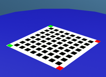
New Calibration pattern for perspective correction

To identify the various features (red, green, black boxes), I generalised the code that I had from my calibration assignment, so that it would work with any color. The caveat is that the adaptive thresholding that I developed works on the grayscale image. But since these images are taken in well lit conditions, that does not really matter. A todo would be to move all the 'magic' constants in the code to a config file so it can be easily modified as and when the lighting conditions change.

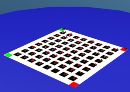
Labeled Calibration pattern (click to enlarge)

Numerically stable solution:

To solve the system of equations and get the projection matrix, I used the least squares technique detailed in last semester's course. It involved calculating the pseudo inverse of a matrix X as [X'(X'X)^-1]. Immidiately, I found that this solution did not work at all for my problem. In the DIP course, our input points lie on two different planes. Here, all my inputs were on a single plane (z=constant). This caused the system to blow up and give me either zero or a very large number as the answer each time. I found that I could get correct results if i randomly perturbed the z values by small amounts.

On Rohit's suggestion, I tried out pseudo inverse using SVD. It worked wonderfully! It turns out that the SVD method is more numerically stable than the regular pseudoinverse techique. To make things better, openCV has already implemented a SVD based solver for a system of linear equations (cvSolve). This not only ensured correct results, but vastly simplified the code (openCV matrix code tends to get messy).

It turns out that the method that I was using to calibrate the camera is fundamentally flawed. The key idea here is that not all 3x4 matrices are calibration matrices. The least squares method tries to fit a 3x4 matrix to a set of observed values. It does not take into consideration the additional constraints that an actual camera imposes on the system. In my case, since all the observed points lie on a single plane, z=0, the components of the projection matrix corresponding to the 'z' coordinate were all near zero. Therefore, the Z coordinate was always being ignored, and all points in the scene would be projected as if their Z component was 0.

I consulted my friend Arnab (PhD student at IITM), who told me to forget writing my own camera calibration code, and use a ready made 'popular camera calibration toolbox'. This motivated me to try out the OpenCV camera calibration method (cvCalibrateCamera). It turns out that this method is surprisingly good, and can calibrate an entire array of cameras at once. This means that if I have 100 images taken using the same camera from different angles, cvCalibrateCamera can extract the intrinsic and extrinsic parameters of the camera all at once. It takes about a minute now to calibrate all the cameras, once I feed in the 3D and corresponding 2D points for each scene.

Furthermore, to verify if the matrices were truly what I was expecting, I wrote a simple voxel renderer which uses a given 3x4 matrix to render the scene. The only gripe of using a 3x4 matrix is that we dont get the relative z values in image space. ie: no easy way of implementing a z-buffer. But the application is sufficient for me to verify that the matrix I get from OpenCV's mystery function is actually a proper camera matrix.

Visualization of a 3x4 projection matrix by rendering a cube

As a final step, I also had to modify a part of Biswarup's original code that took camera coordinates, and allow it to take these 3x4 camera matrices that I had computed. Currently, there are several parts of the original code that will not work until I give them the camera coordinates. One such part (very important) is the final rendering system. It performs a near neighbour search to find cameras approximately corresponding to a given novel view. This step is now completely broken. I will have to check if the camera extrinsics that OpenCV returns will be suitable for this.

Now that I have a set of tools that can capture images, segment them, capture calibration patterns and calibrate the camera setup, it is time to test it out on some synthetic data to see if it really works. I built a simple 3D model by displacing points on a sphere to make it look like a spiked shell. It is a fairly complex model with sharp features, and lots of occlusion. I created a synthetic (animated) turntabe on which I placed a calibration pattern and took a sequence of 27 images around 360 degrees. Then I captured images of the 3D model. This is the input to my tool chain. I have built a set of shell scripts that will simplify the process of 3D reconstruction. The steps I followed are as follows:

• Extract an ordered set of 64 points from each calibration pattern
• Pass these points to the camera calibration routine to get a set of 3x4 camera matrices
• Run a segmentation pass on each image of the object to generate png images with the background set to transparent
• Create a dataset file with the matrices, the extents of the reconstructed object in 3d space, and the paths to the segmented files
• Run the visual hull generation routine on the dataset file to get the final reconstruction

Sample input image, and resultant 3D reconstruction from 27 such images

Thus I now know that the reconstruction system works for perfect input data.

The next stage is to check if the system works for actual data captured by the webcam I am using, which brings me to an interesting point. I recently moved all my experiments to 'Surfel', a slightly older computer in our lab. The strange thing is that OpenCV no longer capures images at 960x720 (which it used to on my earlier machine). So for the moment, I am stuck with using 640x480 images.

One of the key problems which I was aware of from the beginning is that the turntable that I am using has to be aligned at the exact same position while starting calibration image capture, and object capture. Otherwise the 2 sets of images will not correspond to each other and we will have wrong calibration data. To fix this, I used the simplest solution possible. I stuck a marker on the axle of the turntable, and another corresponding marker on the fixed base. Before capturing images, I just manually align these markers. Its not an elegant solution, but it works, as we will see.

I also ran into an unforseen problem when I covered the entire background with a single color (blue) sheet. Earlier, parts of the yellow wall and brown table were visible in the camera and I thought it would be better if I fixed it. But it turns out that the camera performs automatic white balance and saturation control. So, when it sees only one color in the scene, it desaturates everything so that the scene turns gray. This was a hurdle because I could no longer get useful background images. To fix it, I placed a small white strip of paper just within the view frustum of the camera, so that it would not perform such aggressive white balance. It seems to work better now even without any object on the table.

Once I had my test data, I tried to put the images through the same steps I described in the earlier section. Not surprisingly, real data is much harder to work with, and I faced many new problems along the way.

• Extract an ordered set of 64 points from each calibration pattern: This is one of the hardest problems to fix. When a camera captures images, red is no longer red, green is no longer green, and blue, as we have seen, is quite close to gray. I found that my thresholding functions were failing on several calibration images. I introduced backtracking so that the threshold can be lowered if we overshoot and find too many boxes. I also added an option of maximum distance between two boxes, to prevent 2 parts of the same box from being labeled as 2 different boxes. This fixed a lot of errors, but I still had problems with a few images. The system was automatically able to extract calibration parameters for 86 of 89 images. I guess its a good enough result in computer vision, where nothing is certain. For the remaining patterns, I just decided to discard them and their corresponding object images.
• Pass these points to the camera calibration routine to get a set of 3x4 camera matrices: This works fine as long as the previous step does not produce erroneous results, but may just mess up badly if wrong data is passed to it (which is why I test the output matrices using the voxel renderer, to see if any matrices are behaving strangely)
• Run a segmentation pass on each image of the object to generate png images with the background set to transparent: This step is a lot harder as well, because the camera keeps on adjusting the exposure and white balance, drastically desaturating the scene in some images. But I chose to go ahead with a conservative segmentation. This means that it is all right if a few images have a lot of spurious data, but no image should be missing any data. Since the process of finding a visual hull involves volume intersections, any random spurious data that is found in some images will be discarded automatically.

Finally, after all this, I have the visual hull results for the frog dataset:

Sample input image, and resultant 3D reconstruction from 86 images

The output is still a little grainy and is missing very fine features like the tips of the toes of the frog. But I attribute these to the relatively low resolution of captured data (and in part to the slightly bad segmentation results. Better exposure control can fix that). At higher resolutions, things should work just fine.

The real data tests showed that varying exposure levels and lighting conditions can drastically change how the scene looks in different views. This means that a single threshold value is not sufficient for segmentation. Therefore, we need to vary the threshold adaptively based on the input image. To do this, the program asks for the expected ratio of number of foreground pixels to background pixels. This remains relatively constant throughout the process and can be used to set progressively higher thresholds for segmentation.

Non Adaptive Thresholding (left) and Adaptive Thresholding

I have written a set of shell scripts that will automate most of the steps involved in the system. They take as input a set of calibration images, an equal number of object images (all named in alphabetical sequence), a color config file that specifies the colors of the boxes in the calibration pattern, a background image, and a file specifying the dimensions of the visual hull to be constructed. A single script invocation will perform the calibration and segmentation process, select those views that have been properly calibrated and generate a dataset file for the visual hull construction algorithm.

I will be posting results here as and when they are available.

Input data resolution: 960x720, 40 images