In this assignment, you will write code to compute an optimal policy for a given MDP using the algorithms that were discussed in class: Value Iteration, Howard's Policy Iteration, and Linear Programming. The first part of the assignment is to implement these algorithms. Input to these algorithms will be an MDP and the expected output is the optimal value function, along with an optimal policy. You also have to add an optional command line argument for the policy, which evaluates the value function for a given policy instead of finding the optimal policy, and returns the action and value function for each state in the same format.
MDP solvers have a variety of applications. As the second part of this assignment, you will use your solver to find an optimal policy for a team of 2 football players attempting to score a goal against a single opponent in a game of football.
This compressed
directory contains a data directory with sample data for both parts and helper functions to visualise
and test your code. Your code will also be
evaluated on instances other than the ones provided.
All the code you write for this assignment must be in Python 3.8.10. If necessary, you can install Python 3.8.10 for your system from here. Your code will be tested using a python virtual environment. To set up the virtual environment, follow the instructions provided in virtual-env.txt which is included in the compressed directory linked above.
In the mdp folder in data directory, you are given eight MDP instances (4 each
for continuing and episodic tasks). A correct solution for each MDP is
also given in the same folder, which you can use to test your code.
Each MDP is provided as a text file in the following format.
numStates SThe number of states S and the number of actions A will be
integers greater than 1. There will be at most 10,000 states, and
at most 100 actions. Assume that the states are numbered 0, 1,
..., S - 1, and the actions are numbered 0, 1, ..., A - 1. Each
line that begins with "transition" gives the reward and
transition probability corresponding to a transition, where
R(s1, ac, s2) = r and T(s1, ac, s2) = p. Rewards can be
positive, negative, or zero. Transitions with zero probabilities
are not specified. You can assume that
there will be at most 350,000 transitions with non-zero
probabilities in the input MDP. mdptype
will be one of continuing and
episodic. The discount factor gamma is a real number between 0 (included) and 1 (included).
Recall that gamma is a part of the MDP: you must not change it inside your solver! Also recall that it is okay to
use gamma = 1 in episodic tasks that guarantee termination; you will find such an example among the ones given.
To get familiar with the MDP file format, you can view and run generateMDP.py (provided in the
base directory), which is a python script used to generate random MDPs. Specify the number of states
and actions, the discount factor, type of MDP (episodic or continuing), and the random seed as command-line
arguments to this file. Two examples of how this script can be invoked are given below.
python generateMDP.py --S 2 --A 2 --gamma 0.90 --mdptype episodic --rseed 0python generateMDP.py --S 50 --A 20 --gamma 0.20 --mdptype continuing --rseed 0Given an MDP, your program must compute the optimal value
function V* and an optimal policy π* by applying the algorithm that
is specified through the command line. Create a python file
called planner.py which accepts the following command-line arguments.
--mdp followed by a path to the input MDP file, and--algorithm followed by one of vi, hpi, and lp. You must assign a default value out of vi, hpi, and lp to allow the code to run without this argument.--policy (optional) followed by a policy file, for which the value function V^π is to be evaluated.Make no assumptions about the location of the MDP file relative to the current working directory; read it in from the path that will be provided. The algorithms specified above correspond to Value Iteration, Howard's Policy Iteration, and Linear Programming, respectively. Here are a few examples of how your planner might be invoked (it will always be invoked from its own directory).
python planner.py --mdp /home/user/data/mdp-4.txt --algorithm vipython planner.py --mdp /home/user/temp/data/mdp-7.txt --algorithm hpipython planner.py --mdp /home/user/mdpfiles/mdp-5.txt --algorithm lppython planner.py --mdp /home/user/mdpfiles/mdp-5.txtpython planner.py --mdp /home/user/mdpfiles/mdp-5.txt --policy pol.txtNotice that the last two calls do not specify which algorithm to
use. For the fourth call, your code must have a default algorithm from
vi, hpi, and lp that gets
invoked internally. This feature will come handy when your
planner is used in Task 2. It gives you the flexibility to use
whichever algorithm you prefer. The fifth call requires you to
evaluate the policy given as input (rather than compute an
optimal policy). You are free to implement his operation in any
suitable manner.
You are not expected to code up a solver for LP; rather, you
can use available solvers as blackboxes. Your effort will be in
providing the LP solver the appropriate input based on the MDP,
and interpreting its output appropriately. Use the formulation
presented in class. We require you to use the Python
library PuLP. PuLP is convenient to
use directly from Python code: here is
a short
tutorial and here is
a reference. PuLP
version 2.4 is included in the requirements.txt file for the environment.
You are expected to write your own code for Value Iteration and Howard's Policy Iteration; you may not use any custom-built libraries that might be available for the purpose. You can use libraries for solving linear equations in the policy evaluation step but must write your own code for policy improvement. Recall that Howard's Policy Iteration switches all improvable states to some improving action; if there are two or more improving actions at a state, you are free to pick anyone.
It is certain that you will face some choices while implementing your algorithms, such as in tie-breaking, handling terminal states, and so on. You are free to resolve them in any reasonable way; just make sure to note your approach in your report.
The output of your planner must be in the following format and written to standard output, for both modes of operation. Note that, for policy evaluation, V* will be replaced by V^π.
	V*(0)   π*(0)
	V*(1)   π*(1)
	.
	.
	.
	V*(S - 1)   π*(S - 1)
In the data/mdp directory provided, you will find
output files corresponding to the MDP files, which have solutions in
the format above.
Since your output will be checked automatically, make sure you have nothing printed to stdout other than the S lines as above in sequence. If the testing code is unable to parse your output, you will not receive any marks.
Note:
- Your output has to be written to the standard output, not to any file.
- For values, print at least 6 places after the decimal point. Print more if you'd like, but 6 (
xxx.123456) will suffice.- If your code produces output that resembles the solution files: that is, S lines of the form
or evenvalue + "\t" + action + "\n"value + " " + action + "\n"you should be okay. Make sure you don't print anything else.
- If there are multiple optimal policies, feel free to print any one of them.
You are given a python script to verify the correctness of your submission format and solution:
autograder.py. The following are a few examples that can help you understand how to invoke
this script.
python autograder.py --task 1 --> Tests the
default algorithm set in planner.py on the all the MDP
instances given to you in the data/mdp directory.python autograder.py --task 1 --algorithm all
--> Tests all three algorithms + default algorithm on the all the
MDP instances give to you in the data/mdp
directory.python autograder.py --task 1 --algorithm vi -->
Tests only value iteration algorithm on the all the MDP instances
given to you in the data/mdp directory.The script assumes the location of the data
directory to be in the same directory. Run the script to check the
correctness of your submission format. Your code should pass all the
checks written in the script. You will be penalised if your code does
not pass all the checks.
Your code for any of the algorithms should not take more than one minute to run on any test instance.
Problem Description:
You are the manager of a
2-member football team. You want to prepare a strategy that
maximises the chances of scoring goals by doing MDP Planning!
You are tasked with the problem of Half Field Offense - scoring
a goal with two attackers against one defender. The football
half pitch is a 4x4 grid with a goal that is 2 units long. You
have two players - B1 and B2, with possession of the ball, whose
skill levels for different actions are parameterised by p and q
in [0, 0.5] and [0.6, 1]. Note that p and q correspond to
different actions by these players, and are identical for both
players. The opponent has a defender R. You must formulate this
as an MDP and score a goal before you lose possession! The game
ends when the players score a goal, or lose possession,
whichever occurs first.
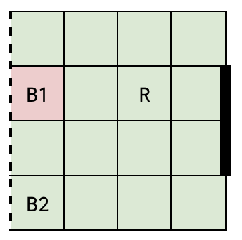
Fig 1: (The playground)
Game positions:
The squares of the grid are numbered from 1 to 16 row-wise. Then the
game position can be specified in the following format --
[B1_square, B2_square, R_square, ball_possession].
Here B1 and B2 are players you control and R is a player from the
opponent team. Ball possession is an integer from 1,2 indicating which
player has the possession.
Thus B1_square, B2_square, and R_square are 2-digit numbers, with a
leading 0 for square numbers below 10.
Note: In the problem statement, you will require x and y coordinates in
some cases, but you can use any origin/axis since only the relative
differences of coordinates matter.
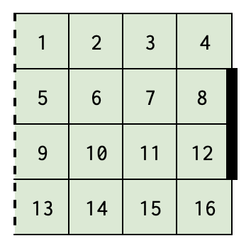
Fig 2: (The positions)
Actions:
Attempt to move one player L, R, U, or D by 1 unit. [0,1,2,3 correspond to L, R, U, D for B1 and 4,5,6,7 correspond to L, R, U, D for B2]
Attempt a pass to your teammate. [8]
Attempt a shot on the goal. [9]
Size of action space = 10.
You are provided with 3 opponent policy files in the data directory that the players can face in the game, giving the probability of the opponent action for each state.
Opponent Policies:
Note that your planner will only compute a policy for the agent (that is, the team of B1 and B2). In order to do so, you will be given R's policy, but you will not compute or change R's policy.
Movement: For moving with the ball (i.e. if movement with the player in possession of the ball), the probability of success in the desired direction is 1-2p and 2p probability of losing possession directly. For moving without the ball there is a 1-p probability of moving in the desired direction and p probability of the game ending (without a goal) directly. If a player chooses to move in a particular direction, there is zero probability of moving in any other direction. The only stochasticity in movement is regarding losing possession directly according to the probabilities described above. If possession is lost, the episode ends. Additionally, If a player goes out of bounds the episode ends.
Tackling: There are two cases in which a tackling situation arises -
A. If a player with possession of the ball and the opponent transition
to a position where they share the same square. The figures below show
an example game position and the actions chosen by the player to reach
this situation. In both of these cases, the probability of the tackle being successful given the move was successful is 0.5. The final probability values are shown in the figure.
Also, note that a tackling situation only arises when the player with the ball attempts to move.
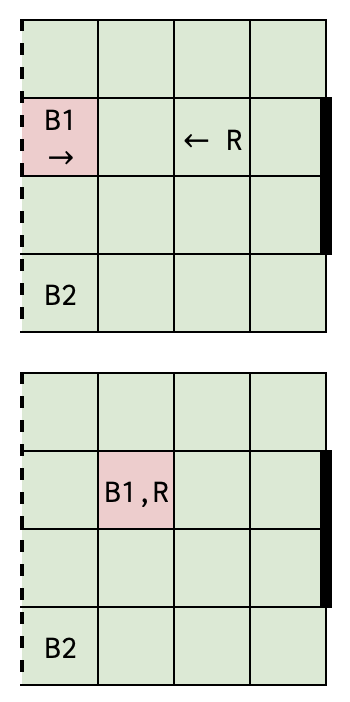
Fig 3, 4: Tackling case A
State: Fig 3
Action: B1 attempts to move right
Opponent Action: Move left from square 7 to 6 according to policy
Outcomes: P(Fig 4 | R moves to square 6) = 0.5 - p, P(episode ends | R moves to square 6) = 0.5 + p
Note: Straight arrows represent player movement. Red squares represent the ball location.
B. If a player with possession of the ball and the opponent are on adjacent squares and they successfully move towards each other, thus swapping squares. The figures below show an example game position and the actions chosen by the player to reach this situation.
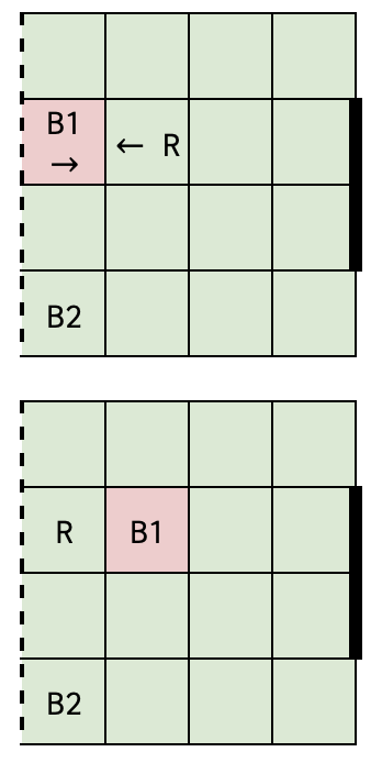
Fig 5, 6: Tackling case B
State: Fig 5
Action: B1 attempts to move right
Opponent Action: Move left from square 6 to 5 according to policy
Outcomes: P(Fig 6 | R moves to square 6) = 0.5 - p, P(episode ends | R moves to square 6) = 0.5 + p
Passing: The probability is a function of the distance from the teammate for passing the ball. If player B1 is on (x1, y1) and B2 is on (x2, y2) then the probability of a successful pass is q - 0.1*max(|x1-x2|, |y1-y2|). This probability is halved if R moves to a square in between B1 and B2, including the squares of B1 and B2. A square is said to be in between two squares if its centre lies on the line joining the centres of the two squares. If a pass fails, then the game ends. While transitioning from one timestep to the next, assume that R moves first and then a pass is attempted by the passer. Thus the above condition must be checked for the new location of R. Example configurations where R is considered to be in between are given below.
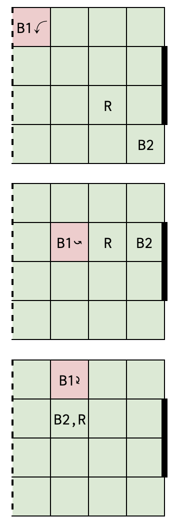
Fig 7, 8, 9: Passing with the opponent in between (Note: Curved arrows represent an attempted pass.)
State: Fig 7
Action: B1 attempts a pass to B2
Opponent Action: Move from some square to square 11 according to policy
Outcomes: P(successful pass | R moves to square 11) = 0.5q - 0.15, P(episode ends | R moves to square 11) = 1.15 - 0.5q
State: Fig 8
Action: B1 attempts a pass to B2
Opponent Action: Move from some square to square 7 according to policy
Outcomes: P(successful pass | R moves to square 7) = 0.5q - 0.1, P(episode ends | R moves to square 7) = 1.1 - 0.5q
State: Fig 9
Action: B1 attempts a pass to B2
Opponent Action: Move from some square to square 6 according to policy
Outcomes: P(successful pass | R moves to square 6) = 0.5q - 0.05, P(episode ends | R moves to square 6) = 1.05 - 0.5q
Shooting: For shooting towards the goal, the probability is a function of the distance of the x coordinate of the shooter. If B1 has the ball and is on (x1, y1) the probability of a goal is q - 0.2*(3-x1). This probability is halved if there is an opponent player in the two squares in front of the goal. If a shot fails, then the game ends. While transitioning from one timestep to the next, assume that R moves first and then a shot is attempted by the shooter. Thus the above condition must be checked for the new location of R.
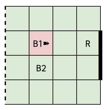
Fig 10: Shooting with the opponent at the goal (Note: Wedged arrows represent an attempted shot.)
State: Fig 10
Action: B1 attempts a shot on goal
Opponent Action: Move from some square to square 8 according to policy
Outcomes: P(goal | R moves to square 8) = 0.5q - 0.2, P(episode ends | R moves to square 8) = 1.2 - 0.5q
Inputs to be provided to students: A list of game positions in the above coordinate system. 3 opponent policy documents with the action probabilities of each action by the opponent from each state in the above format.
Output required from students:
Expected number of goals scored against each of the three opponent policies.
Two graphs indicating the probability of winning starting from position
[05, 09, 08, 1] (shown below) against policy-1 (greedy defense)
[Graph 1]: For p in {0, 0.1, 0.2, 0.3, 0.4, 0.5} and q = 0.7
[Graph 2]: For q in {0.6, 0.7, 0.8, 0.9, 1} and p = 0.3
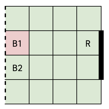
Fig 11: Starting state
Rather than write a solver from scratch for the above game, your job is to translate the above task into an MDP, and use the solver you have already created in Task 1.
Your first step is to write an encoder script which takes as input the player parameters p and q and the opponent policy, and encode the game into an MDP (use the same format as described above).
Your next step is to take the output of the encoder script and
use it as input to planner.py. As
usual, planner.py will provide as output an optimal
policy and value function.
Finally, create a python file
called decoder.py that will take the output from
planner.py along with an opponent file for referring to the order of positions, and convert it into a policy file in the format given above for the game, having
the same format as stated above. Thus, the sequence of encoding,
planning, and decoding results in the computation of an optimal
policy for a player given player parameters and the player parameters and opponent policy
Here is the sequence of instructions that we will execute to obtain your optimal counter-policy.
python encoder.py --opponent data/football/test-1.txt --p 0.1 --q 0.7 > football_mdp.txtpython planner.py --mdp football_mdp.txt > value.txtpython decoder.py --value-policy value.txt --opponent data/football/test-1.txt > policyfile.txtAs stated earlier, note that the planner must use its default
algorithm. You can use autograder.py to verify
that your encoding and decoding scripts produce output in the
correct format, and correctly for the three provided testcases, one for each policy and with different player parameters. Here is how you would use it.
python autograder.py --task 2
The eventual output policyfile will be evaluated by
us (using our own code) to check if it achieves optimal score from
every valid state.
Prepare a short report.pdf file, in which you put
your design decisions, assumptions, and observations about the
algorithms (if any) for Task 1. Also describe how you formulated the
MDP for the Football problem: that is, for Task 2. Finally, include the 2 graphs for Task 2 with your
observations.
Place all the files in which you have written code in a directory named submission. Tar and Gzip the directory to produce a single compressed file (submission.tar.gz). It must contain the following files.
planner.py encoder.py decoder.py report.pdf references.txt Submit this compressed file on Moodle, under Programming Assignment 2.
7 marks are reserved for Task 1 (1 marks for the correctness of your Value Iteration algorithm, and 2.5 marks for Howard's Policy Iteration, Linear Programming each, and 1 mark for the policy evaluation). We shall verify the correctness by computing and comparing optimal policies for a large number of unseen MDPs. If your code fails any test instances, you will be penalised based on the nature of the mistake made.
8 marks are allotted for the correctness of Task 2. Once again, we will run the encoder-planner-decoder sequence on a number of player parameters and verify if the policy you compute is indeed optimal. Within Task 2, 5 marks are assigned for the correctness of the encoder-planner-decoder sequence, and 3 marks are assigned to the graphs and observations.
The TAs and instructor may look at your source code to corroborate the results obtained by your program, and may also call you to a face-to-face session to explain your code.
Your submission is due by 11.55 p.m., Sunday, October 15. Finish working on your submission well in advance, keeping enough time to generate your data, compile the results, and upload to Moodle.
Your submission will not be evaluated (and will be given a score of zero) if it is not uploaded to Moodle by the deadline. Do not send your code to the instructor or TAs through any other channel. Requests to evaluate late submissions will not be entertained.
Your submission will receive a score of zero if your code does not execute on the specified Python and libraries versions in the environment. To make sure you have uploaded the right version, download it and check after submitting (but before the deadline, so you can handle any contingencies before the deadline lapses).
You are expected to comply with the rules laid out in the "Academic Honesty" section on the course web page, failing which you are liable to be reported for academic malpractice.