P = [3.5000 1.1100 1.1100 1.0400 1.0100;
0.5000 0.9700 0.9800 1.0500 1.0100;
0.5000 0.9900 0.9900 0.9900 1.0100;
0.5000 1.0500 1.0600 0.9900 1.0100;
0.5000 1.1600 0.9900 1.0700 1.0100;
0.5000 0.9900 0.9900 1.0600 1.0100;
0.5000 0.9200 1.0800 0.9900 1.0100;
0.5000 1.1300 1.1000 0.9900 1.0100;
0.5000 0.9300 0.9500 1.0400 1.0100;
3.5000 0.9900 0.9700 0.9800 1.0100];
[m,n] = size(P);
Pi = ones(m,1)/m;
x_unif = ones(n,1)/n;
cvx_begin
variable x_opt(n)
maximize sum(Pi.*log(P*x_opt))
sum(x_opt) == 1
x_opt >= 0
cvx_end
R_opt = sum(Pi.*log(P*x_opt));
R_unif = sum(Pi.*log(P*x_unif));
display('The long term growth rate of the log-optimal strategy is: ');
disp(R_opt);
display('The long term growth rate of the uniform strategy is: ');
disp(R_unif);
rand('state',10);
N = 10;
T = 200;
w_opt = []; w_unif = [];
for i = 1:N
events = ceil(rand(1,T)*m);
P_event = P(events,:);
w_opt = [w_opt [1; cumprod(P_event*x_opt)]];
w_unif = [w_unif [1; cumprod(P_event*x_unif)]];
end
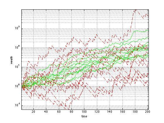
figure
semilogy(w_opt,'g')
hold on
semilogy(w_unif,'r--')
grid
axis tight
xlabel('time')
ylabel('wealth')
Successive approximation method to be employed.
   SDPT3 will be called several times to refine the solution.
   Original size: 35 variables, 21 equality constraints
   10 exponentials add 80 variables, 50 equality constraints
-----------------------------------------------------------------
 Cones  |             Errors              |
Mov/Act | Centering  Exp cone   Poly cone | Status
--------+---------------------------------+---------
 10/ 10 | 2.272e-01  3.277e-03  0.000e+00 | Solved
 10/ 10 | 2.176e-02  3.026e-05  0.000e+00 | Solved
  8/ 10 | 2.785e-03  4.952e-07  0.000e+00 | Solved
  0/  8 | 3.602e-04  8.044e-09  0.000e+00 | Solved
-----------------------------------------------------------------
Status: Solved
Optimal value (cvx_optval): +0.0230783

The long term growth rate of the log-optimal strategy is:
    0.0231

The long term growth rate of the uniform strategy is:
    0.0114