Acknowledgment: This lab assignment is inspired by Project 5: Classification, which is a part of a recent offering of CS188 at UC Berkeley. We thank the authors at Berkeley for making their project available to the public. We also acknowledge the authors of the Kaggle shapes data set, which we use as a part of this assignment.
In this assignment, you will design a multi-class classifier on a set of d-dimensional points: specifically a Perceptron classifier. You will be implementing 2 different types of the multi class perceptron. The initial tasks would be to implement the two different methods to model multi-class perceptron (namely, 1-vs-rest and 1-vs-1) and analyze the results on the given dataset of d dimensional points. Subsequently, you will have to use the same classifier on a new data set of shape images, for which you will also have to design suitable features.
The data set on which you will run your classifiers is a collection
of d-dimensional points which belong to k different classes. The method of generating the data points is as follows:
pick k different corners of a d-dimensional hypercube {1, -1}d. We sample data from a multivariate
gaussian centered at these points. The standard deviation matrix of the multivariate gaussian used is the matrix diag([sigma]*d): that is, the diagonal matrix with all diagonal entries as sigma. These sampled points are your input data.
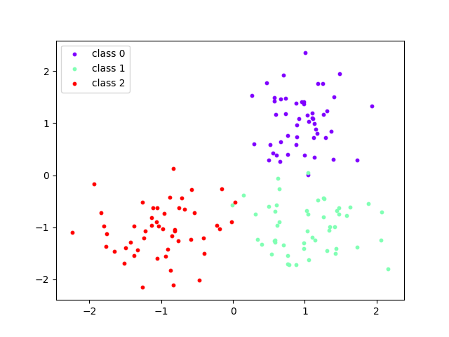
For example, consider the case when d = 2 and k = 3. The hypercube is the square ${[1,1], [1,-1], [-1,1], [-1,-1]}$. Choosing 3 centres from this set, the centres of gaussians are ${[1, 1], [1, -1], [-1,-1]}$. The sampled points are plotted for each of the classes using sigma = 0.5.
Visual Representaion of the 2D Example with 3 classes
In our case, the dimensions of data d = 20, the number of classes k = 10 and the sigma in consideration is 1.5. 100000 such data points along with the corresponding labels (classes) are generated. Out of these 80000 points are kept for training and 20000 points for testing. These are provided in data/D1 directory. For Task 3.1 we will be using limited data from this data set (8000 train and 2000 test), referring to it as D1.2.
This data set contains black and white 50x50 pixel sized images of different shapes. There are 1000 samples of 4 different shapes. We have attached the images as well as the extracted points from the shapes in the data/D2 directory. The extracted shapes will be in the form of a list with value '1' being black and '0' white. The list is generated using a row major scan of the image. The four classes labels are as follows : $['0' : circle, '1' : square, '2' : triangle, '3' : star]$. You can see the variation in the shapes, these variations are due to camera pose differences.
The base code for this assignment is available
in this zip file. You need to use
these files from the classification directory.
| File Name | Description |
| classificationMethod.py | Abstract super class for the classifiers you will write. You should read this file carefully to see how the infrastructure is set up. Do not edit this file. |
| createData.sh | Bash script that runs the perceptron (1 vs rest) classifier on several different sizes of the training set. |
| createGraphIterations.gnuplot | Gnuplot script to plot accuracy versus number of training examples seen. |
| createGraphTraining.gnuplot | Gnuplot script to plot accuracy versus size of the training set. |
| data | Contains the training and test data for both data sets. |
| dataClassifier.py | The wrapper code that will call your classifiers. You will also write your enhanced feature extractor here. |
| answers.txt | Blank text file for you to enter answers from Task 2 and Task 3. |
| perceptron1vr.py | The file where you will write your first perceptron (1 vs rest) classifier. |
| perceptron1v1.py | The file where you will write your second perceptron (1 vs 1) classifier. |
| autograder.py | The file we will be using to test your assignment. Do not edit this file. |
| samples.py | I/O code to read in the classification data. Do not edit this file. |
| util.py | Code defining some useful tools, that will save you a lot of time. Do not edit this file. |
| references.txt | In which you will note down every site/resource to which you have referred while working on this assignment. |
There exist two broad techniques to solve the multi-class classification problem (see this link for an overview). We will be implementing and comparing both these techniques in this assignment.
A Perceptron keeps a weight vector $w^y$ corresponding to each
class $y$ ($y$ is a suffix, not an exponent). Given a feature list
$f$ (a vector with the same number of dimensions as the weight
vectors), the perceptron computes the class $y$ whose weight vector
is most similar to the input vector $f$. Formally, given a feature
vector $f$ (in D1 (the point itself) and in D2 (a list of indicators for pixels being on)), we score each class $y$ with
$$score(f, y) = \Sigma_i f_i w_i^y$$ where $i$ iterates over the dimensions in the data. Then we choose the class with
the highest score as the predicted label for data instance $f$. In the code, we will represent $w^y$ as a Counter (defined in the file util.py).
In the basic multi-class Perceptron, we scan over the training data one instance at a time. When we come to an instance $(f,y)$, we find the label with highest score: $y\prime=argmax_{y\prime\prime}score(f,y\prime\prime)$, breaking ties arbitrarily. We compare $y\prime$ to the true label $y$. If $y\prime=y$, we have correctly classified the instance, and we do nothing. Otherwise, we predicted $y\prime$ when we should have predicted $y$. That means that $w_y$ has scored $f$ lower, and/or $w_{y\prime}$ has scored $f$ higher, than what would have been ideal. To avert this error in the future, we update these two weight vectors accordingly: $$w_y=w_y+f,$$ and $$w_{y\prime}=w_{y\prime} - f.$$
In this technique the perceptron maintains $S = (k * (k-1)) / 2$ weights vectors, one for each distinct pair of classes, each weight vector of the same dimension as the number of features. Every weight vector corresponding to $w_{(y, y')}$ can be thought of as a binary classifier between classes $y$ and $y'$. When we come to an instance $(f,y)$, assuming some ordering among the classes; $$w_{(y, y')} \cdot f > 0 \implies max(y, y')$$ is the class that gets a vote and $$w_{(y, y')} \cdot f \leq 0 \implies min(y, y')$$ is the class that gets a vote. While guessing the class of an unknown data sample we do $S$ such votes and the class that receives the maximum votes is predicted, with ties settled arbitrarily.
Here we need to analyse all class pairs separately; that is, for each distinct (y, y') pair, we consider only data points belonging to these two classes, and perform a binary perceptron algorithm like update (as taught in class) on them. (Note : No need to actually separate the training samples according to class pairs, you can do this in the same loop while iterating through all the data points).
In this task, you have to implement the 1-vs-rest multi-class Perceptron
classifier. Fill out code in the train() function at the
location indicated in perceptron1vr.py. Using the addition,
subtraction, and multiplication functionality of
the Counter class in util.py, the perceptron
updates should be relatively easy to code. Certain implementation
issues have been taken care of for you in perceptron1vr.py,
such as the following.
weights data structure. This can be accessed using self.weights in the train() method.Counter of weights.Run your code with the following command.
python dataClassifier.py -c 1vr -t 80000 -s 20000
This will print out a host of details, such as the classifier that
is being trained, the training set size, if enhanced features are
being used (more on this in Task 4), etc. After this, the classifier
gets trained for a default of 3
iterations. dataClassifier.py would then print the
accuracy of your model on the train and test data sets.
The -t option passed to the Perceptron training code
specifies the number of training data points to read in from memory,
while the -s option specifies the size of the test set
(the train and test data sets are mutually independent). Since
iterating over 100000 points may take some time, you
can use 1000 data points instead while developing and testing your
code. However, note that all our evaluations will involve train
and test data sets with 100000 points.
Evaluation: Your classifier will be evaluated by for its accuracy on the test set after the Perceptron has been trained for the default 3 iterations. You will be awarded 3 marks if the accuracy exceeds 70%, otherwise 2 marks if accuracy exceeds 60%, otherwise 1 mark if accuracy exceeds 50%, otherwise 0 marks. You can run the autograder script to test your final implementation.
AutoGrader Script for this task is as follows.
python autograder.py -t 1
One of the problems with the perceptron is that its performance is
sensitive to several practical details, such as how many iterations
you train it for, the order you use for the training examples, and how
many data points you use. The current code uses a default value of 3
training iterations. You can change the number of iterations for the
perceptron with the -i iterations option. In practice,
you would use the performance on the validation set to figure out when
to stop training, but you don't need to implement this stopping
criterion for this task.
Instead, you need to analyse and comment on how the test and train accuracy changes (1) as the total number of data points seen during training change, and (2) as the total size of the training set changes. See details below.
Variation with number of training data points 'seen': In this sub-task, you need to plot the train and test accuracy as increasing numbers of data points are 'seen' (that is, a point is examined to determine whether an update needs to be made to the Perceptron1vr, or the point is already correctly classified, and so no update is needed) by the classifier.
You have been provided helper code for this purpose:
the train() function in perceptron1vr.py
writes <examples seen>,<train and test
accuracy> as a comma-separated pair into the
file perceptron1Iterations.csv and perceptron1IterationsTrain.csv 20 times in an
iteration. The plotting
script createGraphIterations.gnuplot uses this csv
file to create the required plot and save it in a file by
name plot_iterations.png. You can modify either of
the two code files mentioned above to modify the plot being
generated. Feel free to experiment with the various switches and
write a description of your observations and a description of the
nature of the plot in the file answers.txt in
plain text.
Below are commands to generate the required graph.
python dataClassifier.py -c 1vr -t 8000 -s 2000 -v
gnuplot createGraphIterations.gnuplot
Variation with training set size in each iteration: Here, you will see the influence of training set size on the accuracy of train and test set, when trained for the same number of iterations.
Every time dataClassifier.py is run, it writes a
comma-separated pair of numbers<training set
size>,<accuracy>for the train and the test
sets to files perceptron1vr_train.csv
and perceptron1vr_test.csv. Use createData.sh
(supplied in the zip file) to run the perceptron training on 100, 200,
300, ..., 1000 examples. Create a plot
named plot_training.png by
running createGraphTraining.gnuplot. Below are
commands to generate the required graph.
./createData.sh
gnuplot createGraphTraining.gnuplot
Append your observations and description of the plot obtained in
the file answers.txt (to which you had already
written in the previous sub-task). Additionally, answer the following
question.
Note: The bash script to generate the data for the graph might take a long time to run. You are advised to proceed to subsequent tasks while the script is running.
Evaluation: Sub-tasks 1 and 2 will be evaluated for a total of 2 marks, with the plots and the corresponding explanations and answers all taken into consideration.
In this task, you have to implement the One-vs-One multi-class Perceptron
classifier. Here you can think of each weight vector as a binary classifier and so the updates to multiclass perceptron are just updates to multiple relevant binary perceptrons. Fill out code in the train() function at the
location indicated in perceptron1v1.py. Using the addition,
subtraction, and multiplication functionality of
the Counter class in util.py, the perceptron
updates should be relatively easy to code. Certain implementation
issues have been taken care of for you in perceptron1v1.py,
such as the following.
Counter of weights.Run your code with the following command.
python dataClassifier.py -c 1v1 -t 80000 -s 20000
Run an experiment using only 800 data points for training while testing on 8000 data points (D1.2). Do this for both perceptron1vr and perceptron1v1. Use the following calls.
python dataClassifier.py -c 1vr -t 800 -s 8000
python dataClassifier.py -c 1v1 -t 800 -s 8000
Describe the result in the answers.txt. Also mention the test accuracies
obtained while both the perceptron algorithms running on 80000 train and 20000 test,
that is the full D1 data set. You need to compare the test accuracies acquired by the two
algorithms for both the datasets and state and explain your observations.
Evaluation: Your classifier will be evaluated by for its accuracy on the test set (from D1) after the Perceptron has been trained for the default 3 iterations. You will be awarded 3 marks if the accuracy exceeds 75%, otherwise 2 marks if accuracy exceeds 65%, otherwise 1 mark if accuracy exceeds 55%, otherwise 0 marks. 1 mark is reserved for writing the analysis in answers.txt.
AutoGrader Script for this task is as follows.
python autograder.py -t 3
This task will require using the data set D2. It requires using the One-vs-rest classifier (Perceptron1vr) implemented in Task 1.
Building classifiers is only a small part of getting a good system working for a task. Indeed, the main difference between a good classification system and a bad one is usually not the classifier itself, but rather the quality of the features used. Run the Perceptron1vr algorithm implemented in Task 1 on the D2 data set using this command.
python dataClassifier.py -c 1vr -t 800 -s 200 -k 4 -d d2
So far, we have only used the simplest possible features:
the identity of each pixel (being on/off).
You will see a good accuracy (>90%) achieved. Your task is to use at most 5 features i.e. 5 float/int valued features and achieve as much accuracy as possible. You will need to extract more useful features from the data than the pixel values and use only them as features. The EnhancedFeatureExtractorDigit()
in dataClassifier.py is your new playground. When
analysing your classifiers' results, you should look at some of your
errors and look for characteristics of the input that would give the
classifier useful information about the label.
As a concrete illustration, consider the data you have used. In each training point (a inary matrix corresponding to an image), consider the number of separate, connected regions of white pixels. This quantity, although it does not vary across shapes, is an example of a feature that is not directly available to the classifier from the per-pixel information. Further you can add features that cumulatively describe all the per pixel values. You can also try analysing edges and corners.
If your feature extractor adds new features such as the quantity
described above (think of others, too!), the classifier will be able
exploit them. Note that some features may require non-trivial
computation to extract, so write efficient and correct code. Add your
new features for the shape data set (D2) in
the EnhancedFeatureExtractorDigit() function.
We will test your classifier with the following command.
python dataClassifier.py -c 1vr -t 800 -s 200 -k 4 -d d2 -f
Evaluation: If your new features give you a test accuracy exceeding 85% using the command above, you will get 3 marks. Accuracy exceeding 70% will get 2 marks and accuracy more than 50% will get 1 mark
Note: Using comments in your code, briefly explain the working of your EnhancedFeatureExtractorDigit().
AutoGrader Script for this task is as follows.
python autograder.py -t 4
You are expected to work on this assignment by yourself. You may
not consult with your classmates or anybody else about their
solutions. You are also not to look at solutions to this assignment or
related ones on the Internet. You are allowed to use resources on the
Internet for programming (say to understand a particular command or a
data structure), and also to understand concepts (so a Wikipedia page
or someone's lecture notes or a textbook can certainly be
consulted). However, you must list every resource you have
consulted or used in a file named references.txt,
explaining exactly how the resource was used. Failure to list all
your sources will be considered an academic violation.
Be sure to write all the observations/explanations in the answers.txt
We have mentioned wherever there is such a requirement. Find the keyword 'answers.txt'
in the page.
Place all files in which you have written code in or modified in a
directory named la1-rollno, where rollno
is your roll number (say 12345678). Tar and Gzip the directory to
produce a single compressed file
(say la1-12345678.tar.gz). It must contain the
following files.
perceptron1vr.py perceptron1v1.py answers.txt dataClassifier.py plot_iterations.png plot_training.png references.txt Submit this compressed file on Moodle, under Lab Assignment 1.