CS 335: Lab Assignment 2

In this assignment, you will design layers required to build both a feed-forward neural network (also popularly known as a Multilayer Perceptron classifier) and the Convolution Neural Networks. Feed-forward NNs and CNNs form the basis for modern Deep Learning models. However, the networks with which you will experiment in this assignment will still be relatively small compared to some of modern instances of neural networks.

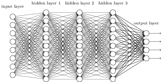
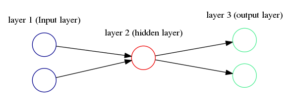
An artificial neural network with 3 hidden layers
(Image source: http://neuralnetworksanddeeplearning.com/images/tikz41.png.)

Data Sets

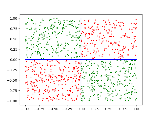
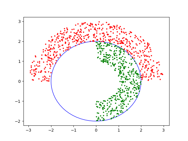
To test your code, you are provided a set of toy examples (1 and 2 below), each a 2-dimensional, 2-class problem. You are also provided tools to visualise the performance of the neural networks you will train on these problems. The plots show the true separating boundary in blue. Each data set has a total of 10,000 examples, divided into a training set of 8000 examples, validation set of 1000 examples and test set of 1000 examples.

Data set 3 is the MNIST data set collection of images handwritten digits.

Data set 4 is the CIFAR-10 data set collection of images of commonly seen things segregated into 10 classes.

XOR Data (Left)

The input X is a list of 2-dimensional vectors. Every example X_i is represented by a 2-dimensional vector [x,y]. The output y_i corresponding to the i^th example is either 0 or 1. The labels follow XOR-like distribution. That is, the first and third quadrant has same label (y_i = 1) and the second and fourth quadrant has same label (y_i = 0) as shown in Figure 1.

Semicircle Data (Right)

The input X is a list of 2-dimensional vectors. Every example X_i is represented by a 2-dimensional vector [x,y]. The output y_i corresponding to the i^th example is either 0 or 1. Each set of label (y_i = 1 and y_i = 0 ) is arranged approximately on the periphery of a semi circle of unknown radius R with some spread W as shown in Figure 2.

MNIST Data

We use the MNIST data set which contains a collection of handwritten numerical digits (0-9) as 28x28-sized binary images. Therefore, input X is represented as a vector of size 784. These images have been size-normalised and centred in a fixed-size image. MNIST provides a total 70,000 examples, divided into a test set of 10,000 images and a training set of 60,000 images. In this assignment, we will carve out a validation set of 10,000 images from the MNIST training set, and use the remaining 50,000 examples for training.

CIFAR 10 Data

We use the CIFAR-10 data set which contains 60,000 32x32 color(RGB) images in 10 different classes. The 10 different classes represent airplanes, cars, birds, cats, deer, dogs, frogs, horses, ships, and trucks. There are 6,000 images of each class. These 60,000 images are divided into a test set of 10,000 images and a training set of 50,000 images. In this assignment, we will carve out a validation set of 10,000 images from the CIFAR-10 training set, and use the remaining 40,000 examples for training.

In this assignment, we will code a feed-forward neural network and convolution neural network from scratch using python3 and the numpy library.

Code

The base code for this assignment is available in this compressed file. Below is the list of files present in the Lab2_base directory.

All data sets are provided in the datasets directory.

Understanding the code

We start with building the neural network framework. The base code for the same is provided in nn.py and layer.py.

nn.py. The base code consists of the NeuralNetwork class which has the following methods.

• __init__ : Constructor method of the NeuralNetwork class. The various parameters are initialised and set using this method. The description of various parameters can be seen in file nn.py.
  
  
• addLayer : Method to add layers to the neural network.
  
  
• train: This method is used to train the neural network on a training data set. Optionally, you can provide the validation data set as well, to compute validation accuracy while training. Further description on various input parameters to the method are available in the base code.
  
  
• computeLoss: This method takes as input the neural network activations of the final layer predictions and the actual labels Y and computes the squared error loss for the same.
  
  
• computeAccuracy: This method takes as input the predicted labels in one hot encoded form, predLabels, and the actual labels Y and computes the accuracy of the prediction. The two toy data sets will require neural nets with two outputs, and MNIST and CIFAR neural nets would have 10 outputs. In each case the output with the highest activation will provide the label.
  
  
• validate: This method takes as input the validation data set, validX and validY, and computes the validation set accuracy using the currently trained neural network model.
  
  
• feedforward: This method takes as input the training data features, X, and does one forward pass across all the layers of neural network.
  
  
• backpropagate: This method takes as input the training labels and activations produced by forward pass, and does one backward pass across all the layers of neural network.
  
  

layers.py. The base code consists of various Layer classes, each of which have the following methods.

• __init__: This method takes as input the various parameters need to construct a particular layer of neural net (for example, a fully connected layer would required input and output nodes as parameters). Some layers contain self.weights and self.biases (numpy multi dimensional arrays) which are initialized using a normal distribution with mean 0 and standard deviation 0.1. The specific dimensions of these are given in layers.py.
  
  
• forwardpass: Needs to be implemented.
  
  
• backwardpass: Needs to be implemented.
  
  

Methods you need to implement

You will only have to write code inside the following functions. You need to implement these functions for all the layers in the layer.py.

• forwardpass: This method takes as input activation from previous layer X, and returns new activations w.r.t. this layer. The activations must be returned as a list of numpy arrays.
  NOTE: Remember to follow same convention as specified in the comments of the layers.py file. Also, you might need to save the outgoing summation of weights * feautres + biases calculated during the forward pass to be used in backpropagation
  
  
• backwardpass: This method takes as input the activations of previous layer (activation_prev) and partial derivatives of the error w.r.t. current layer activations(delta), and updates the weights and biases of the current layer. It returns as output the partial derivatives of the error w.r.t previous layer activations.
  NOTE: You must implement backpropagation based on sigmoid activation everywhere. Recall that sigmoid(x) = 1 / (1 + e^-x).
  
  

Layers: Explanation and References

• Fully Connected Layer: This layer contains weights in form of in_nodes X out_nodes . Forward pass in such a layer is simply matrix multiplication of activations from previous layer and its weights and addition of bias to it. A_new = A_old X Curr_Wts + Bias. Similarly, backpropagation updates can be obtained by simple matrix multiplications.
  
  
• Convolution Layer: This layer contains weights in form of numpy array of form (out_depth, in_depth, filter_rows, filter_cols). Forward pass in such layer can be obtained from correlation of filter with the previous layer for all its depths and addition of biases to this sum. Backwardpass for such a system of weights results in another convolution that you need to figure out.
  
  
• AvgPooling Layer: This layer is essentially used to reduce the weights used in convolution. It downsamples the previous layer by a factor stride and filter (in our case both can be assumed to the same). While downsampling one could have used many operations, including taking mean, median, max, min, etc,. Here we take the Average operation for downsampling. This doesn't effect the depth of the input. Forward pass in such layer can be obtained by taking Mean in a grid of elements of size = filter_size. Backwardpass for such a system just upsamples the numpy multidimensional array, scaling them by same factor that was used in downsampling.
  
  
• Flatten Layer: This layer is inserted to convert 3d structure of convolution layers to 1d nodes required for fully connected layers.
  
  

Refer to this link and to this link for further clarifications on how to implement forward and backward propagation across average-pooling and convolution layers

Following are some key numpy functions that will speed up the computation: tile, transpose, max, argmax, repeat, dot, matmul. To perform element-wise product between two vectors or matrices of the same dimension, simply use the * operator. For further reference on these functions refer to numpy documentation.

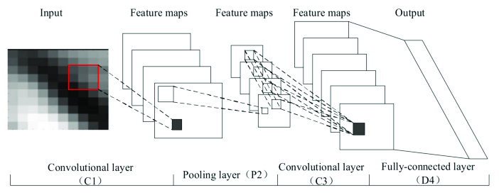
A CNN with 2 Convolution layers, 1 Pooling Layer and 1 Fullyconnected layer. Flatten Layer b/w C3 and D4 is implicit in the figure
(Image source: https://www.researchgate.net/figure/Structure-of-a-typical-convolutional-neural-network-CNN_fig3_323938336.)

Task 1: Forward Pass (1 + 1 + 2 = 4 Marks)

In this task, you will complete the feedforward methods in layers.py file.

Testing your feed-forward network

To test your feed forward network implementation, run the following code.

Task 2: Backpropagation implementation(1 + 1 + 3 + 4 + 2 = 11 Marks)

In this task, you are required to complete the backwardpass() methods in layers.py file. You should (will have to) use the matrix form of the backpropagation algorithm for quicker and more efficient computation. Also, see Task 2.5 before tweaking models for remaining tasks, as you have to report neural networks with minimal topologies.

Evaluation over Data Sets

Your backpropagation code will be tested on toy data sets (tasks 2.1 and 2.2) and 2 marks will be awarded if you get test accuracies over 90% on each of the toy data sets.

Task 2.1: XOR Data set (1 Marks)

Complete taskSquare() in tasks.py. To test your backpropagation code on this data set, run the following command

Task 2.2: SemiCircle Data set (1 Marks)

Complete taskSemiCircle() in tasks.py. To test your backpropagation code on this data set, run the following command.

Task 2.3: Compute Accuracy over MNIST (using Feed-Forward Neural Network) (3 marks)

The MNIST data set is given as mnist.pkl.gz file. The data is read using the readMNIST() method implemented in util.py file.

Your are required to instantiate a NeuralNetwork class object (that uses FullyConnectedLayers) and train the neural network using the training data from MNIST data set. Choose appropriate hyper parameters for the training of the neural network. To obtain full marks, your network should be able to achieve a test accuracy of 90% or more across many different random seeds. You will get 1.5 marks if your test accuracy is below 90%, but still exceeds 85%. Otherwise, you will get 1 mark if your test accuracy is at least 75%.

Complete taskMnist() in tasks.py. To test your backpropagation code on this data set, run the following command.

Task 2.4: Compute Accuracy over CIFAR (using Convolution Neural Network) (4 marks)

The CIFAR-10 data set is given in cifar-10 directory. The data is read using the readCIFAR10() method implemented in util.py file.

Your are required to instantiate a NeuralNetwork class object (with at least one convolutional layer) and train the neural network using the training data from CIFAR data. You are required to choose appropriate hyperparameters for the training of the neural network. To obtain full marks, your network should be able to achieve a test accuracy of 35% or more. You will get 2 marks if your test accuracy is below 35%, but still exceeds 30%. Otherwise, you will get 1 mark if your test accuracy is at least 25%. Note that we require lower accuracies than is reported in the literature as CNNs take a lot of time to train. Moreover, we have added code to reduce the size of training, test and validation set (see tasks.py). You are free to choose the size of data to use for training, testing and validation as you see fit. For submission remember to save the weights is the file model.npy (look nn.py train() function for more details) for your trained model and also uncomment line 90 in tasks.py. Also list all your hyperparameters and the random seed used (seedValue) for training on this task (in a file named observations.txt), so we can reproduce your results exactly.
NOTE: You will require lot of time to train (at least 4-5 hrs) in order to get the above accuracies. So start working on this assignment as early as possible, leaving 1-2 days for training alone.

Complete taskCifar10() in tasks.py. To test your backpropagation code on this data set, run the following command.

Task 2.5: Describe the results (2 marks)

In this task, you are required to report hyperparameters (learning rate, number of hidden layers, number of nodes in each hidden layer, batchsize and number of epochs) of Neural Network for each of the above 4 tasks that lead to minimal-topology neural networks that pass the test: that is, with the minimal number of nodes you needed for each task. For example, in case of a linearly separable data set, you should be able to get very high accuracy with just a single hidden node. Write your observations in observations.txt. Also, explain the observations.

Submission

You are expected to work on this assignment by yourself. You may not consult with your classmates or anybody else about their solutions. You are also not to look at solutions to this assignment or related ones on the Internet. You are allowed to use resources on the Internet for programming (say to understand a particular command or a data structure), and also to understand concepts (so a Wikipedia page or someone's lecture notes or a textbook can certainly be consulted). However, you must list every resource you have consulted or used in a file named references.txt, explaining exactly how the resource was used. Failure to list all your sources will be considered an academic violation.

Remember to test your solution before submission using the autograder provided.

Place these four files (and additionally references.txt) in a directory (la-2-rollno), and compress it to be la2-rollno.tar.gz where rollno is your roll number (say 12345678, then Final compressed file would be la2-12345678.tar.gz) and upload it on Moodle under Lab Assignment 2.