
Acknowledgment: This lab assignment is partly based on Project 5: Classification, which is a part of a recent offering of CS188 at UC Berkeley. We thank the authors at Berkeley for making their project available to the public.
Ensemble Learning, a form of meta-learning, is a machine learning paradigm where multiple learners are trained to solve the same problem. In this assignment, you will code up the meta-learning algorithms Bagging (short for Bootstrap Aggregating) and Boosting (specifically AdaBoost). These meta-learners will operate on the Perceptron as a base learner, which you have already worked on in Lab Assignment 1.
(Image source: https://scroll.in/magazine/872431/sofar-sounds-a-unique-initiative-allows-musicians-and-audiences-to-discover-one-another-in-india)
The data set on which you will run your meta-learning algorithms is a collection of handwritten numerical digits (\(0-9\)). However we have decided to have you solve only a two-class problem. Hence, classes \(0-4\) have the label -1, and classes \(5-9\) have the label 1. Details about your tasks, and the files you must submit as a part of this assignment, are mentioned in the sections below.
The base code for this assignment is available
in this zip file. You need to use
these files from the ensembling directory.
| File Name | Description |
| answers.txt | Blank text file for you to enter answers from Task 2 and Task 3. |
| autograder.py | This is used for testing your Task 2 and Task 3 |
| bagging.py | The file where you will write your bagging classifier. |
| boosting.py | The file where you will write your boosting classifier. |
| classificationMethod.py | Abstract super class for the classifiers you will write. You should read this file carefully to see how the infrastructure is set up. Do not edit this file. |
| createBaggingData.sh | Bash script that runs the classifiers on several different counts of weak classifiers. |
| createBoostingData.sh | Bash script that runs the classifiers on several different counts of weak classifiers. |
| createGraphBagging.gnuplot | Gnuplot script to plot accuracy versus number of weak classifiers. |
| createGraphBoosting.gnuplot | Gnuplot script to plot accuracy versus number of weak classifiers. |
| data.zip | Contains the training, validation and test data sets. |
| dataClassifier.py | The wrapper code that will call your classifiers. |
| perceptron.py | The file where you will write your perceptron classifier. |
| samples.py | I/O code to read in the classification data. Do not edit this file. |
| util.py | Code defining some useful tools, that will save you a lot of time. Do not edit this file. |
In this task, you have to implement the 2-class Perceptron
classifier. Fill out code in the train() function at the
location indicated in perceptron.py. Using the addition,
subtraction, and multiplication functionality of
the Counter class in util.py, the perceptron
updates should be relatively easy to code. You can and are advised to
use code from Lab Assignment 1, while keeping in mind you are solving
a 2-class problem.
Run your code with the following command.
python dataClassifier.py -c perceptron -t 1000 -s 1000
The classifier should be able to get an accuracy of 65% - 70%.
Bagging and boosting are in the spirit of learning a strong classifier from a set of weak classifiers. The main difference lies in the way they choose data sets for training each base learner.
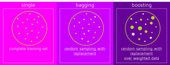
(Image source: https://quantdare.com/wp-content/uploads/2016/04/bb2-1150x441.png)
Given a standard training set \(D\) of size \(N\), bagging generates \(M\) new training sets \(\{D_m\}^M_{m=1}\), each of size \(N^{\prime}\), by sampling from \(D\) uniformly at random and with replacement. By sampling with replacement, some observations may be repeated in each \(D_m\). These data sets are significantly different from each other as only about 63% of the original data set will appear in any of \(D_m\) if \(N=N^{\prime}\).
The data sets generated \(D_1, D_2, \dots, D_M\) are fed to individual weak learners \(h_1, h_2, \dots, h_M\), respectively. This brings out the most important characteristic of bagging which gives it a definitive advantage over boosting in terms of speed, that you can train weak learners in parallel.
Finally, for a new data point \(x\), it is fed into each of the weak learners \(\{h_m\}^M_{m=1}\). The outputs from each weak learner \(y^{\prime}_1, y^{\prime}_2, \dots, y^{\prime}_M\) is then polled to find the label whose count is maximum. In other words,
\( y = sign(\sum^{M}_{m=1}y^{\prime}_m) \).
The AdaBoost algorithm in each iteration trains a new weak learner with the same data set \(D\) but with associated weights for each sample: \(w_1, w_2, \dots, w_N\). After training, each misclassified point is weighed up so that in the next training iteration the weak learner classifies them correctly. Also a set of hypothesis weights \(z_1, z_2, \dots, z_M\) are computed for each \(h_1, h_2, \dots, h_M\) respectively which determine the effectiveness of the corresponding hypotheses.
The output for a new data point \(x\) is obtained by thresholding a weighted summation of the labels \(y^{\prime}_1, y^{\prime}_2, \dots, y^{\prime}_M\) produced by each weak learner weighed according to the hypothesis weights:
\( y = sign(\sum^{M}_{m=1}y^{\prime}_m \times z_m) \)
Refer to Section 18.10 of Russell and Norvig (2010) for a detailed description.
Your task is to implement the 2-class bagging classifier with
perceptron as the weak learner. Fill out code in the train() and classify() functions at the location indicated in bagging.py.
train() should contain the code to sample points from the data set with replacement and then training the weak classifier using the sampled data set. classify() should contain the code to get the labels from individual classifiers and then running voting to find the majority.
Note: We do not expect you to write parallel code for this task.
Run your code with the following command.
python dataClassifier.py -c bagging -t 1000 -s 1000 -r 1 -n 20
Evaluation: Your classifier will be evaluated for its accuracy on the test set after the Bagging algorithm has been run with weak learners trained for the default 3 iterations. You will be awarded 3 marks if the accuracy exceeds 75%, otherwise 2 marks if the accuracy exceeds 73%, otherwise 1 mark if the accuracy exceeds 71%, otherwise 0 marks.
The autograder Script for this task is as follows.
python autograder.py -t 2
In this task you have to implement the 2-class adaboost classifier with
perceptron as the weak learner. Fill out code in the train() and classify() function at the location indicated in boosting.py. Also you will have to fill the sample_data() function in perceptron.py which converts a weighted data set to an unweighted one. Remember that perceptron algorithm doesn't work with weights assigned to individual samples. The size of the sampled data set should be set to within 0.5 - 1.5 times the size of original data set.
train() should contain the code to compute the weights for each data point after training the weak classifier. classify() should contain the code to get the labels from individual classifiers and then have weighted summation to get the final output.
Run your code with the following command.
python dataClassifier.py -c boosting -t 1000 -s 1000 -b 20
Evaluation: Your classifier will be evaluated for its accuracy on the test set after the AdaBoost algorithm has been run with weak learners trained for the default 3 iterations. You will be awarded 4 marks if the accuracy exceeds 75%, otherwise 3 marks if the accuracy exceeds 74%, otherwise 2 marks if accuracy exceeds 73%, otherwise 1 mark if the accuracy exceeds 71%, otherwise 0 marks.
The autograder script for this task is as follows.
python autograder.py -t 3
Variation with number of weak classifiers: Here, you will see the influence of number of weak classifier on the accuracy of validation set, when trained for the same number of iterations.
Every time dataClassifier.py is run, it writes a
comma-separated pair of numbers—<number of classifiers>,<accuracy>—for the train, the validation and the test
sets to files {classifier}_train.csv, {classifier}_val.csv
and {classifier}_test.csv. Use create{classifier}Data.sh
(supplied in the zip file) to run the algorithm with 1, 3, 5, 7, 9, 10, 13, 15, 17, 20 weak classifiers. Create a plot
named plot_{classifier}.png by
running createGraph{classifier}.gnuplot. Below are
commands to generate the required graph.
./create{classifier}Data.sh gnuplot createGraph{classifier}.gnuplotNote: It takes quite a lot of time to generate the numbers, so keep 1 day just for running the scripts before the final submission deadline.
Feel free to experiment with the various switches and write a description of your observations and a description of the nature of the plot in the file answers.txt in plain text for both the algorithms. Additionally, answer the following question.
You are expected to work on this assignment by yourself. You may
not consult with your classmates or anybody else about their
solutions. You are also not to look at solutions to this assignment or
related ones on the Internet. You are allowed to use resources on the
Internet for programming (say to understand a particular command or a
data structure), and also to understand concepts (so a Wikipedia page
or someone's lecture notes or a textbook can certainly be
consulted). However, you must list every resource you have
consulted or used in a file named references.txt,
explaining exactly how the resource was used. Failure to list all
your sources will be considered an academic violation.
Be sure to write all the observations/explanations in the answers.txt file.
We have mentioned wherever there is such a requirement. Find the keyword 'answers.txt'
in the page.
Place all files in which you have written code in or modified in a
directory named la3-rollno, where rollno is
your roll number (say 12345678). Tar and Gzip the directory to produce
a single compressed file (say la3-12345678.tar.gz). It
must contain the following files.
perceptron.py bagging.py boosting.py answers.txt plot_bagging.png plot_boosting.png references.txt Submit this compressed file on Moodle, under Lab Assignment 3.