In this assignment, you will implement Value Iteration, which is an MDP planning algorithm. The input to the algorithm is an MDP and the expected output is the optimal value function, along with an optimal policy. MDP solvers have a variety of applications. As a part of this assignment, you will use your solver to find the shortest path between a given start state and an end state in a maze.

Data

This compressed directory contains 2 folders: mdp and maze. In the mdp folder, you are given three MDP instances, along with a correct solution for each which you can use to test your code in Task 1. In the maze folder, you are given 10 maze instances which you can use to test your code in Task 2 and Task 3. Your code will also be evaluated on instances other than those provided.

MDP file format

Each MDP is provided as a text file in the following format.

The number of states \(S\) and the number of actions \(A\) will be integers greater than 0. Assume that the states are numbered \(0, 1, \dots, S - 1\), and the actions are numbered \(0, 1, \dots, A - 1\). Each line that begins with "transition" gives reward and transition probability corresponding to one transition where \(R(s1,ac,s2)=r\) and \(T(s1,ac,s2)=p\). Rewards can be positive, negative, or zero. Transitions with zero probabilities are not specified. The discount factor gamma is a real number between \(0\) (included) and \(1\) (included).

\(st\) is the start state, which you might need for Task 2 (ignore for Task 1). \(ed1\), \(ed2\),..., \(edn\) are the end states (terminal states). For continuing tasks with no terminal states, this list is replaced by -1.

To get familiar with the MDP file format, you can view and run generateMDP.py (provided in the base directory), which is a python script used to generate random MDPs. Change the number of states and actions, the discount factor, and the random seed in this script in order to understand the encoding of MDPs.

Maze file format

Each maze is provided in a text file as a rectangular grid of 0's, 1's, 2, and 3's. An example is given here along with the visualisation.

1 1 1 1 1 1 1 1 1 1 1
1 0 0 0 0 0 0 0 1 0 1
1 1 1 0 1 0 1 1 1 0 1
1 3 0 0 1 0 1 0 1 0 1
1 1 1 1 1 0 1 0 1 0 1
1 0 0 0 1 0 1 0 0 0 1
1 1 1 0 1 0 1 0 1 1 1
1 0 0 0 0 0 0 0 1 0 1
1 1 1 1 1 1 1 0 1 0 1
1 0 0 0 0 2 0 0 0 0 1
1 1 1 1 1 1 1 1 1 1 1

Here 0 denotes an empty tile, 1 denotes an obstruction/wall, 2 denotes the start state and 3 denotes an end state. In the visualisation below, the white square is the end position and the yellow one is the start position.

The figure on the right shows the shortest path.

Section 1: Solving MDPs

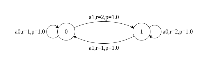
In this assignment we will consider both continuing and episodic MDPs. In a continuing MDP, the agent lives for ever and values correspond to an infinite discounted sum. Below is an example of one such MDP with 2 states and 2 actions. If the discount factor is taken as 0.9, it is seen that the optimal value attained at each state is 20. The optimal policy takes action a1 from state 0, and action a0 from state 1. This MDP is available as mdpfile01.txt.

In episodic tasks, some states are terminal states and the agent's life ends as soon as it enters any terminal state. By convention, the value of the terminal state is taken as zero and conceptually, there is no need for policies to specify actions from terminal states.

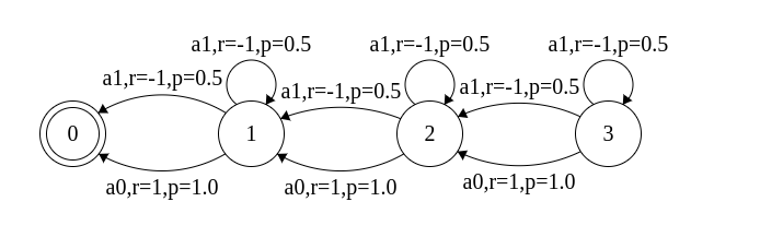
The figure below corresponds to an episodic task with 4 states, with state 0 being terminal. Take the discount factor as 0.9. From each of the states 1, 2, and 3, action a0 deterministically takes the agent left, while action a1 either carries it left or keeps it in the same state (each with probability 0.5). a0 gives positive rewards, while a1 gives negative rewards. It is not hard to see that a0 is the optimal action from each of the non-terminal states. Under the optimal policy, the value of state 1 is 1, the value of state 2 is 1 + 0.9 = 1.9, and the value of state 3 is 1 + 0.9 + 0.81 = 2.71. This MDP is available as mdpfile02.txt

Value Iteration

Value iteration is a simple, iterative algorithm, which is specified in the slides provided in class. Assume \(V^{0}\), the initial value vector, has every element as zero. Terminate when for every state \(s\), \(|V^t(s) - V^{t - 1}(s)| <= 10^{-16}\). You can assume that at this point, \(V^{t}\) is the optimal value function. An optimal policy can be obtained by taking greedy actions with respect to the optimal value function.

You will have to handle two novel aspects as a part of your implementation. First, observe that only those transitions that have non-zero probabilities are given to you in the input MDP file. In the Bellman Optimality Operator, it should suffice for you to iterate only over next states that have a non-zero probability of being reached. It would consume additional time to unnecessarily iterate over zero-probability transitions; make sure your internal data structures and code implement the efficient version.

How should you handle the end states? Fix their value to be zero, and do not update it. However, you will still use its (zero) value on the RHS of the Bellman Optimality update.

Task 1 - Implementing Value Iteration (6 marks)

Given an MDP, your code must compute the optimal value function \(V^{\star}\) and an optimal policy \(\pi^{\star}\). Its output, written to standard output, must be in the following format.

The first \(S\) lines contain the optimal value function for each state and the action taken by an optimal policy for the corresponding state. The last line specifies the number of iterations taken by value iteration (the value of variable \(t\) in the pseudocode upon termination). In the data directory enclosed, you will find three solution files corresponding to the MDP files, which have solutions in the format above. Naturally, the number of iterations you obtain need not match the number provided in the solution, since it will depend on your implementation. The optimal policy also need not be the same, in case there are multiple optimal policies. Make sure the optimal value function matches, up to 6 decimal places.

Since your output will be checked automatically, make sure to print nothing to stdout other than the \(S + 1\) lines as above in sequence. Print the action taken from the end state (if any) as -1.

Implement value iteration in any programming language of your choice (provided it can be tested on the SL2 machines), taking in an MDP file as input, and producing output in the format specified above. The first step in your code must be to read the MDP into memory; the next step to perform value iteration; and the third step to print the optimal value function, optimal policy, and number of iterations to stdout. Make sure your code produces output that matches what has been provided for the three test instances.

Create a shell script called valueiteration.sh, which will be called using the command below.

Here mdpFileName will include the full path to the MDP file; it will be the only command line argument passed. (If, say, you have implemented your algorithm in C++, the shell script must compile the C++ file and run the corresponding binary with the MDP it is passed.) The shell script must write the correct output to stdout. It is okay to use libraries for data structures and for operations such as finding the maximum. However, the logic used in value iteration must entirely be code that you have written.

Section 2: Solving a maze using MDPs

In this section your objective is to find the shortest path from start to end in a specified maze. The idea is to piggyback on the value iteration code you have already written in Section 1. We will consider two types of environments in a maze: Deterministic and Stochastic. In a deterministic environment, the agent moves exactly as specified by the action which essentially reduces to a deterministic MDP. However in a stochastic environment, the agent may move to some cell other than the one implied by the specified action.

Note: In the following tasks, assume that any invalid move doesn't change the state e.g., a right move doesn't change the state if there's a wall on immediate right of the current cell. This is applicable for both deterministic and stochastic environments.

Task 2 - Deterministic Maze (3 marks)

Your first step is to encode a deterministic maze as an MDP (use the same format as described above). Then you will use valueiteration.sh to find an optimal policy. Finally, you will simulate the optimal policy on the maze in a deterministic setting to extract a path from start to end. Note that in a deterministic maze, this path also corresponds to the shortest possible path from start to end. Output the path as: A0 A1 A2 . . .
Here "A0 A1 A2 . . ." is the sequence of moves taken from the start state to reach the end state along the simulated path. Each move must be one of N (north), S (south), E (east), and W (west). See, for example, solution10.txt in the maze directory, for an illustrative solution.

To visualise the maze, use command: python visualize.py gridfile

To visualise your solution use command: python visualize.py gridfile pathfile

Create a shell script called encoder.sh that will encode the maze as an MDP and output the MDP. You can use any programming language of your choice (provided it can be tested on the SL2 machines). The script should run as: ./encoder.sh gridfile > mdpfile

We will then run ./valueiteration.sh mdpfile > value_and_policy_file

Also create a shell script called decoder.sh that will simulate the optimal policy and output the path taken between the start and end state given the file value_and_policy_file and the grid. The output format should be as specified above. You can use any programming language of your choice (provided it can be tested on the SL2 machines). The script should run as follows.

./decoder.sh gridfile value_and_policy_file

Task 3 - Stochastic Maze (3 marks)

Consider a stochastic environment where the agent is able to make a correct move with a probability \(p\) and chooses any random valid move (which doesn't result in a collision) with probability \(1-p\). You can think of this as an environment which causes information loss with a probability \(1-p\), thus allowing the agent to receive correct action only with probability \(p\).

As an example, consider the yellow cell in the image below. For this cell, valid moves are - east and west. In our stochastic setting, any given valid action (east or west) will lead to a correct move with a probability \(p\) and a random move (east or west) with probability \(1-p\). Which, for instance, means a west action will lead to a west move with probability \(p+(1-p)/2\) and an east move with probability \((1-p)/2\). Any other actions will not change the position (as they are invalid moves). In this task you will make necessary changes to your code from Task 2 so that your implementation is able to handle such a case.

Specifically, add an optional command line argument to your encoder.sh script which specifies the probability \(p\) with which the agent moves correctly. Make sure that you set the default value of \(p\) to be 1 (to make it compatible with Task 2). Make any other required changes in your code to encode the maze as a stochastic MDP. After all the changes, your script should run as: ./encoder.sh gridfile p > mdpfile

Similarly add the optional command line argument \(p\) to your decoder.sh. Make necessary changes such that while simulating the optimal policy, the agent moves to correct cell (implied by the optimal action) with a probability \(p\) and to a random valid neighbouring cell with probability \(1-p\). After you've done this, your decoder script should run as follows.

./decoder.sh gridfile value_and_policy_file p

The main difference between the deterministic and stochastic mazes is that in the latter, the sequence of state-actions visited by following an optimal policy could be different on different runs, due to randomness. Ideally we should average over several runs to estimate the expected number of steps to complete the maze from the start state. However, in this task, we only ask that you simulate and plot a single run, which we take as representative. You can set the random seed to 0.

Run your code with grid20.txt maze and \(p=0.2\) and visualise the path using visualize.py script as mentioned above. Save the visualisation as path.png. Also, run your code with the grid10.txt maze and different values of \(p\), ranging from 0 to 1 (both included) and plot the number of actions required to reach the exit from the given start state as a function of \(p\). Save this plot as plot.png. Write and explain your observations from the two plots in observations.txt.

Evaluation

Note that we do not have the usual autograder scripts for this assignment. We will run your code on the MDP and maze instances provided to you. Your code should compute the correct answer for all these instances. We will also inspect your code and run it on other test cases to make sure you have implemented your algorithms correctly. If your code fails any test instances, you will be penalised based on the nature of the mistake made. For Task 3, we will also check your path.png and plot.png figures, as well as your observations.

Submission

You are expected to work on this assignment by yourself. You may not consult with your classmates or anybody else about their solutions. You are also not to look at solutions to this assignment or related ones on the Internet. You are allowed to use resources on the Internet for programming (say to understand a particular command or a data structure), and also to understand concepts (so a Wikipedia page or someone's lecture notes or a textbook can certainly be consulted). However, you must list every resource you have consulted or used in a file named references.txt, explaining exactly how the resource was used. Failure to list all your sources will be considered an academic violation.

Place all the files in which you have written code in a directory named la6-rollno, where rollno is your roll number (say 12345678). Tar and Gzip the directory to produce a single compressed file (say la6-12345678.tar.gz). It must contain the following files.

1. valueiteration.sh
2. encoder.sh
3. decoder.sh
4. path.png
5. plot.png
6. observations.txt
7. references.txt
8. Any other files required to run your scripts

Submit this compressed file on Moodle, under Lab Assignment 6.