Acknowledgement: This lab assignment is prepared from several resources: the MNIST data set, the Keras library, and the Tensorflow Playground. We thank the creators of these resources for making them available to the public.
We continue with the same task we investigated in Lab Assignment 2: designing classifiers for the OCR of scanned handwritten digits. In this assignment, you will design a feed-forward neural network (also popularly known as a Multilayer Perceptron) classifier for the task. Feed-forward neural networks form the basis for modern Deep Learning models. However, the networks with which you will experiment in this assignment will still be relatively small compared to some of today's instances.
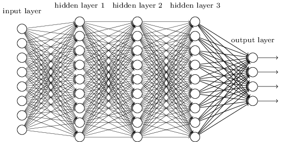
An artificial neural network with 3 hidden layers
(Image source: http://neuralnetworksanddeeplearning.com/images/tikz41.png.)
We continue to use the MNIST dataset which contains a collection of handwritten numerical digits (0-9) as 28x28-sized greyscale images. These images have been size-normalized and centered in a fixed-size image. For the previous assignment, we used only 1000 images for training the Perceptron. Since a neural network has many neurons that need to be trained (and consequently, many tunable parameters), it typically needs a lot more data to be trained successfully. MNIST provides a total 70,000 examples, divided into a test set of 10,000 images and a training set of 60,000 images. In this assignment, we will carve out a validation set of 10,000 images from the MNIST training set, and use the remaining 50,000 examples for training.
The ideal assignment to understand the working of neural networks would be to code up the backpropagation algorithm, taking into account variations in activation functions and loss functions. However, there are several libraries available that provide optimised implementations of such low-level primitives, and allow the programmer to instead focus on high-level network design. In this assignment, we will use Keras, which is a high-level library developed over Tensorflow and Theano for quick prototyping.
The base code for this assignment is available
in this zip file. Below is the list of files
present in the lab03-base directory.
| File Name | Description |
neural-network.py |
This file contains base code in Keras to create a simple 1-layer neural network. |
generic-plot.gnuplot |
A generic gnuplot script. |
experiments.sh |
A simple script for running experiments. |
playground.zip |
This file is to be unzipped to create a local (edited) copy of the Tensorflow playground for Task 4. |
Just like the previous assignment, we have provided you a basic
skeleton of code to get you started. In the file
neural-network.py, you have everything needed to create,
train, and evaluate the performance of a neural network. The comments
provided in this file, along with
the Keras documentation, should help
you develop an understanding of the steps involved. Run the code
using the following command.
python neural-network.py
You will see the progress of the neural network training on your terminal. Here is the meaning of the terms you see.
You must have noticed that one needs to set several parameters—such as the number of hidden layers, the number of neurons in each hidden layer, the non-linearity or activation function to be used, etc. These quantities are known as the hyper-parameters of the network. They need to be specified by the user creating the neural network model.
In this task, you will evaluate the performance of your network for varying values of hyperparameters. Keeping the rest of the values constant (and equal to the default values), adjust the values of parameters as described below. Find the performance (accuracy) of your model on the validation set and plot a trend graph for each of the following.
neural-network.py to do so. The file
expects one command-line argument by default. Edit corresponding lines
of code in the file to read in the required hyperparameter.
You can use experiments.sh as a template to run your
experiments. A generic gnuplot script to plot your graphs is present
in the file generic-plot.gnuplot. Print values of the
parameter you are varying (batch size, hidden layers, learning rate)
in the first column, and the corresponding validation accuracy in the
second column, in a comma-separated file (which is read and plotted by
generic-plot.gnuplot). Plot using this command.
gnuplot generic-plot.gnuplot
Save the graphs
as batch-size.png, num-hidden-layers.png,
and learning-rate.png. Write a brief description of the
variation observed in each graph and your hypothesis explaining the
variation in your own words. Should accuracy alone be the criterion
deciding a parameter setting? What could be other considerations in
practice? Put your answers in plain text
in task1-answers.txt.
Evaluation: Each plot will be evaluated for 1 mark (for the correctness of the graph, as well as the interpretation), and the final architecture and its accuracy will also be evaluated for 1 mark.
One of the key steps to improve the performance of your classifier is to identify the misclassifications being made by the model. This step can be used to identify the classes that need to be separated (say, by creating new features or by training on more examples). In this task, you will create a 'confusion matrix' of the performance of your model on the validation set.
A confusion matrix is a square matrix with one row and one column for each label. Each cell in the matrix contains the number of instances whose true label is that of row of the cell, but which our classifier predicted as the label corresponding to the column of the cell. Therefore, if an example with true label 'x' gets classified as 'y' by our classifier, it would contribute to the total in cell (x, y). Since the diagonal elements represent the number of points for which the predicted label is equal to the true label, and off-diagonal elements are those that are mislabeled by the classifier, the higher the diagonal values of the confusion matrix, the better. Below is an illustrative confusion matrix for a 3-class classification problem.
| Predicted label | |||||
|---|---|---|---|---|---|
| 1 | 2 | 3 | |||
| True label |
1 | 130 | 1 | 10 | |
| 2 | 10 | 110 | 16 | ||
| 3 | 12 | 7 | 90 | ||
Representative confusion matrix for 3 labels.
For this exercise, set the hyperparameters of the network to the values that resulted in the maximum validation accuracy in Task 1. Train your model and evaluate the performance of your model on the validation set. Now use the predictions of your model and the true labels of the validation set to create the 10x10 confusion matrix. Note that the (i,j)th element of the array should correspond to the number of examples belonging to class i, that your network classified as j.
Copy or print your confusion matrix to the
file task2-answers.txt. Also answer the following
questions in task2-answers.txt.
The main purpose of creating a machine learning model is to obtain good performance on unseen test data (not part of the training set of the model). If a model does this, it is said to generalise well to unknown test sets.
In the case of neural networks, training is really the modification
of weights and biases of individual neurons. Every weight and bias is
a 'free parameter' of the model and can be 'tuned' as the network is
trained to do correct classifications. How many parameters does your
neural network created in the Task 2 have? Write down the number and
show the calculation to obtain it in the
file task3-answers.txt.
With so many parameters, would it always be the case that the
neural network you have created generalises well? Find out by training
the neural network on just the first 1000 of the 50,000 training
examples, for 500 iterations. Write down the loss and the
accuracy on the training set as well as the test set for the trained
network; leave your answer in the
file task3-answers.txt.
If you have performed the experiments correctly, you will notice that it is almost as though the network is memorising the training set, without understanding digits well enough to generalise to the test set. This is known as 'overfitting'. There are several ways to prevent overfitting, such as reducing the number of parameters (layers, neurons) in the network, training on more data, etc. Other techniques such as early stopping, regularisation of weights, and dropout, are beyond the scope of this assignment.
Evaluation: Each question above carries 1 mark.
Each neuron in a neural network defines regions in feature space corresponding to the different predictions. By using more neurons and hidden layers, we can create increasingly complex boundaries for these regions.
In this task, we want you to play around with neural networks in an edited version of the Tensorflow Playground, and to classify the `spiral' and the 'flower' data sets using as few layers (and number of neurons in those layers) as possible. Under the "Data" panel on the left, 'spiral' is the data set in the second row and second column, while 'flower' is the data set in the third row and first column. Use only the features X1 and X2, without regularisation. Feel free to choose your activation function, learning rate and other hyperparameters. Instructions to run the visualisations are as follows.
Download
the edited
version of the Tensorflow Playground. After unzipping the folder,
run the following commands:
cd playgroundnpm run cleannpm run buildnpm run serveThis should get the server running on localhost:8080 (enter this in your browser).
Experiment with various topologies in order to get a (near-)perfect
classification of the data points, using a minimal architecture. You
need to attach screenshots of the model that does complete
classification. Save the screenshots
as classify-spiral.png
and classify-flower.png. Also, explain how your chosen
architecture and hyperparameters 'work' on each data set. Do so
in task4-answers.txt.
Evaluation: 1 mark for each data set. Note that you must achieve a test loss of 0.07 or less.
Extra (no credit): Play around with the code to generate your own data sets. You might want to clear the cache of your browser before running this code afresh, since it is possible that saved cookies will not allow your changes to be visible after you edit the code.
You are not done yet! Place all files in which you have written code or modified in a directory named your roll number (say 12345678). Tar and Gzip the directory to produce a single compressed file (12345678.tar.gz). It must contain the following files.
neural-network.py batch-size.png num-hidden-layers.png learning-rate.png classify-spiral.png classify-flower.png task1-answers.txt task2-answers.txt task3-answers.txt task4-answers.txt citations.txt (If you have used any on-line code or resources, cite them in this file.)Submit this compressed file on Moodle, under Lab Assignment 3.