Acknowledgement: This lab assignment is based on the Weka open source Machine Learning package. We thank the creators of this resource for making it available to the public.

There is a wide spectrum of methods for supervised learning, each with its own inductive bias. Examples include linear methods, neural networks, decision trees, and nearest-neighbour classifiers. "Meta-learning" algorithms such as boosting and bagging use individual learners as blackboxes, and can often improve the accuracy of predictions. It exceeds the scope of this introductory course to study each of these methods in depth. However, you can become familiar with many of them with just a few clicks of the mouse. Weka is a user-friendly software meant for quick prototyping of different machine learning algorithms.

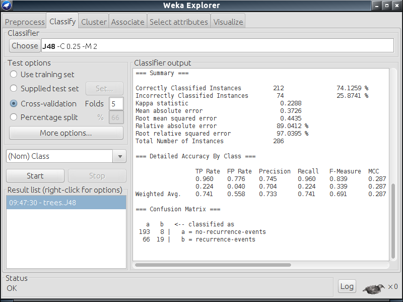
Screenshot of Weka

This assignment will introduce you to Weka. Your tasks will involve training decision trees, neural networks, and decision stumps (which are ensembles of "short" decision trees).

Software and Data Sets

We have already installed Weka on SL2 machines, and so all you have to do to get started is to run the command

on your terminal. If, however, you encounter an error, you can run it from a jar file that we provide you. The jar file for Weka, the manual, and the data sets for this assignment are all available in this zip file. Unzip the file and put it on your Desktop. If simply running weka didn't work, you can also open the Weka GUI by running the following command.

Also export the location of the "weka.jar" file in the CLASSPATH variable.

After opening the GUI, feel free to explore the various options: data sets, tasks, learning algorithms, and evaluation metrics. You can achieve the same functionality through the command line. For example, in order to run the J48 algorithm (decision trees) on the breast-cancer.arff data set, and see the results of 5-fold cross-validation, run this command from the terminal.

Here 't' specifies the training data set and 'x' stands for n-way cross validation. You can separately visualise the data set characteristics using this command.

Before moving on, make sure you can launch the Weka GUI, and also run it from the command line.

Data files are read in by Weka in the Attribute-Relation File Format (ARFF). See, for example, "breast-cancer.arff". The first few uncommented lines describe attributes (which we also call features) and their ranges. Then the data is specified, one row at a time: list of attributes and label.

Tasks and Evaluation

This assignment consists of 4 tasks, each requiring you to run some experiments and answer some questions. You will submit your answer to each question as a separate text file: make sure you include all the commands used in the experiments corresponding to that task (or, if necessary, a script to generate the commands). You will also submit supporting graphs and data. When there is no specific mention of the evaluation metric to use, apply 5-fold cross-validation.

Task 1: Post-pruning of Decision Trees (2 marks)

In this first task, you are required to work on the "diabetes.arff" data set. You have to apply the J48 classification algorithm with -split-percentage as 80. This option will create a training data set with 80% of the points, and use the remaining points for testing.

The focus of this exercise is to visualise the effect of the parameter called the 'Confidence Factor'. Once the tree has been built (nodes with fewer than minNumObj data points are not split), a further pass of pruning is performed by applying the confidence factor. The confidence factor may be viewed as how confident the algorithm is about the training data. A low value leads to more pruning; a high value keeps the model close to the original tree built from the training data (the parameter is used in estimating error probabilities at leaves).

Run experiments with the following values of the confidence factor (default 0.25, maximum 0.5), with the train/test split as specified.

• Confidence Factor: 0.002 , 0.008 , 0.02 , 0.08 , 0.1 , 0.2 , 0.3 , 0.4 , 0.5.

For these values, record both the training and test accuracy, and plot a graph between Accuracy (for both training and test data set in same graph) and Confidence Factor. A generic gnuplot script to plot your graphs is present in the file generic-plot.gnuplot, where you have to write the output file name and input file name. Plot using this command.

gnuplot generic-plot.gnuplot

Save the graphs as confidence-factor.png. Explain the patterns you see in the graph in q1-answer.txt.

Task 2: Comparing decision trees and neural networks (4 marks)

In this task you will apply both J48 and the MultilayerPerceptron to the following data sets: "bank-data.arff" and "mnist-small.arff". Note down the accuracy (5-fold cross-validation) while keeping the number of epochs for the Multilayer Perceptron as 3. Keep all the other parameters at their default settings.

What accuracy do these methods achieve on "bank-data.arff" and "mnist-small.arff"? Can you think of reasons to explain their relative accuracy on these data sets? What are the properties of the data sets? Describe the decision tree model that is learned in each case; how are the models learned for the two data sets different? Note down your observations in q2-answer.txt.

Note: By default Weka takes the last column in the input arff file to be the target class, but this is not the case in "mnist-small.arff". Use the option -c first while training on this data set.

Task 3: Analysis of training time (2 marks)

In this task, you will apply both J48 and MultilayerPerceptron on the following data sets.

• iris.arff
• vote.arff
• soybean.arff
• unbalanced.arff
• segment-challenge.arff
• supermarket.arff
• mnist-small.arff
• mnist-large.arff

Our main object of interest is the time taken to build the decision tree and neural network models in each case. Since the experiments could take time, keep the split percentage as 80, and the number of epochs for the MultilayerPerceptron as 2 for "mnist-small.arff" and as 1 for "mnist-large.arff". Plot a common graph of time (for building the model, not testing) versus the size of the data set, with one curve for each classifier. Also plot a second, similar graph of test accuracy versus the size of the data set.

Submit the data for the graphs, as well as the graphs themselves, with the following names: q3-time.csv, q3-accuracy.csv, q3-time-graph.png, and q3-accuracy-graph.png. Write down your observations from the two graphs. Is either J48 or MultilayerPerceptron always the method of choice? If yes, which one? If not, why? Provide your answers in q4-answer.txt.

Note: Since some of these experiments could take considerable time to run, proceed to your next task while these runs are finishing.

Task 4: Boosting Decision Stumps (2 marks)

Decision stumps are degenerate decision trees with only one split (sometimes we also grow random trees—in which features are chosen at random to split—to two or some small number of levels, combined in an ensemble called a random forest). Naturally the expressive power of decision stumps is very limited. However, decision stumps can be combined into an ensemble, whose collective classification accuracy could be much higher. This task is meant to demonstrate the phenomenon of combining multiple weak learners into a strong learner, using a meta-learning algorithm called Boosting.

For this final task, you will work with DecisionStump and LogitBoost on the "musk.arff" data set. LogitBoost constructs an additive model, starting with a single decision stump, and then training each subsequent decision stump to optimally remedy the errors made by the current group of decision stumps (or the ensemble). Members of the ensemble are also weighted; the prediction made for a test query is the weighted majority of the predictions made by the ensemble. While running LogitBoost, you need to specify DecisionStump as the base learner.

Note down the accuracies for DecisionTump and Logitboost in q5-answer.txt. How many iterations does LogitBoost need to reach 90% accuracy? Feel free to try out and comment on more variations. You might like to refer to the Wikipedia page on Boosting.

Submission

You are not done yet! Place all files in which you have written code or modified in a directory named "la-4" concatenated with your roll number (say la4-12345678). Tar and Gzip the directory to produce a single compressed file (la4-12345678.tar.gz). It must contain the following files.

1. q1-answer.txt
2. q1-Confidence-factor.csv
3. q1-Confidence-factor.png
4. q2-answer.txt
5. q3-answer.txt
6. q3-time.csv
7. q3-accuracy.csv
8. q3-time-graph.png
9. q3-accuracy-graph.png
10. q4-answer.txt

Submit this compressed file on Moodle, under Lab Assignment 4.