The traveling salesperson problem (TSP) asks the following question: "Given a list of cities and the distances between each pair of cities, what is the shortest possible route that visits each city and returns to the origin city?" It is an NP-hard problem in combinatorial optimization, important in operations research and theoretical computer science. In this assignment you will implement hill climbing to solve TSP. We will consider only the Euclidean version of TSP, in which the cities all lie on a 2-dimensional plane. Each city will have (x,y) coordinates, and the euclidean distance between two cities will be the weight of the edge connecting them.
(image source: https://xkcd.com/399/.)
hill climb You have to make changes in |
|
An input instance of a TSP problem (for example, see berlin52.tsp in
the data folder) has one line corresponding to each city. This line
specifies the index of the city, the x coordinate, and the y
coordinate. In hillClimb.py , you will find the Node
data structure. A node contains the index of a city, along with its
x and y coordinates.
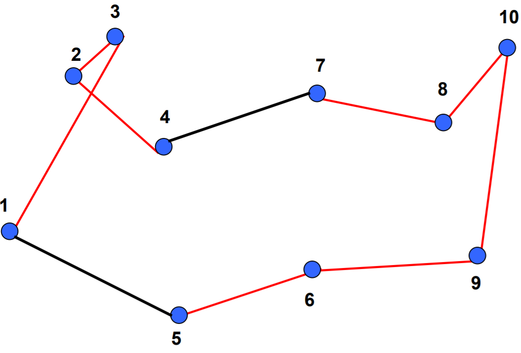
A tour is defined as a permutation of indices of nodes a1, a2, ..., an (where ai is the index of node provided in the input file). Suppose b1, b2, ..., bn is a tour: it means the salesperson starts the tour at b1, then goes to b2, and so on until finally returning to b1 from bn. So a tour is just a list of node indices.
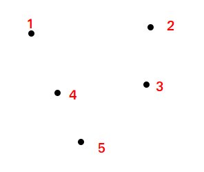
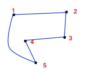
For example, some tours in the instance shown below (left) are [1, 2, 3, 4, 5] (middle) and [2, 1, 3, 4, 5] (right). Any rotated version or mirror image of a tour is the same tour (e.g. 1,2,3,4,5 is the same as 2,3,4,5,1 which is the same as 3,4,5,1,2 and so on. Similarly 1,2,3,4,5 is same as 5,4,3,2,1).
In the code, the following variables, functions and data structures are implemented for your convenience.
As presented in class, you will consider the 2-neighbourhood of nodes to perform hill climbing. You will also implement two non-trivial initialisation routines, which should help hill climbing find better solutions.
Not that although we apply "hill climbing" in this assignment, we only maintain tour lengths, which we aim to minimise. It would be unnatural to consider the negative of tour lengths and find a maximum. So we'll stick with minimising tour lengths. Consequently, although we call our method hill climbing, we'll be performing valley-descending.
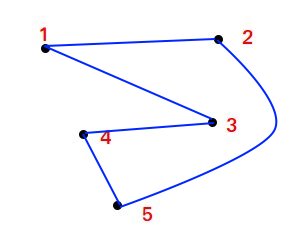
Two tours are called 2-neighbours if one can be obtained from the other by deleting two edges and adding two edges. For example, the two tours shown below are 2-neighbours of each other.
For a given tour, generate a list of all its 2-neighbours (also
sometimes called 2-opt neighbours). You will be implementing the
function generate2optNeighbours(tour). Here tour is a list
of indices of cities/nodes. When you fill out the function, it should
return a list of tours. For
example, generate2optNeigbours called on [1, 2, 3, 4]
should return [ [2, 1, 3, 4], [3, 2, 1, 4], [1, 3, 2, 4]]. The order
of the tours does not matter. In principle it is a good idea not to
have rotated/mirrored copies of tours in the list returned, as they
add unnecessary complexity to the algorithm. However, your code will
still work if the list returned
by generate2optNeighbours(tour) has such copies. For
example, the above call might as well have returned ( [[4,1,3,2],
[3,2,1,4], [2,1,3,4],[1,3,2,4]], where [4,1,3,2] is just the rotated
version of [1,3,2,4]).
Hint: there is a simple trick to generate 2-neighbours quickly. See if reversing some substring of the tour list gives you something useful.
Use python3 hillClimb.py -h to get familiar with
different command line options that you can use. After making changes
to generate2optNeighbours(tour)
in hillClimb.py, use the following command to test the
function.
python3 hillClimb.py --file tsp4.tsp --task 1 This call should return [[4, 1, 3, 2], [1, 4, 3, 2], [3, 1, 4, 2], [4, 3, 1, 2],[1, 4, 3, 2], [4, 3, 1, 2]] or some variation involving rotations and mirror images. Also run tests with other instances, if you would like to make sure your code is correct.
You can generate your own instance and use it for printing the 2-neighbours, using this command.
python3 hillClimb.py --cities 'number of cities' --r1seed 'random seed for generating city distances' --r2seed 'random seed for tour generation' --task 1Note that the '--r1seed' random seed will be used to generate random coordinates for the given number of cities, and the '--r2seed' random seed will be used for creating a random initial tour. For example,
python3 hillClimb.py --cities 10 --r1seed 2 --r2seed 3 --task 1
will generate the 'tsp10' file for 10 cities with random coordinates in your current directory and will use it to generate 2-neighbours. If you are using an existing file, then there is no need to pass the '--cities' and '--r1seed' options. Just use this command.
python3 hillClimb.py --file 'filename' --r2seed 'seed value' --task 1These command line options for generating new TSP instances or using existing ones are common to all tasks.
For submission, run this command.python3 hillClimb.py --file data/tsp10.tsp --r2seed 1 --task 12optNeighbours.txt in your directory, which you need to submit for Task 1.
You will implementing the
function hillClimbFull(initial_tour), which must return
two things:
For example, hillClimbFull([1, 2, 3, 4, 5]) on some instance might return something like
[12.2, 11, 7.7, 5.6, 5.5, 3.8], [2, 3, 1, 5, 4].
As an intermediate step, you might find it useful to implement
a hillClimbUtil(Tour) function that undertakes a
single step of hill climbing: that is, takes as input a tour,
generates all its 2-neighbours, and chooses the minimum length one.
You will use the function that you have implemented in Task 1 to
generate 2-neighbours. (In other tasks, too, feel free to modularise
your code by creating your own functions.)
By running
python3 hillclimb.py --file data/berlin52.tsp --r2seed 1 --task 2 For submission, run python3 hillClimb.py --submit --task
2, which will generate task2_submit.png. This
experiment runs your hill climbing code on st70.tsp, and uses
5 different random tour initialisations. The graph is plotted
for each of the initialisations. This graph will be used for your
evaluation.
The choice of initial tour before applying hill climbing can make a significant difference in the final tour found. In the next two tasks, we will investigate different approaches to pick a 'good' initial tour.
Under this approach, given a starting node A, a tour is constructed in the following manner. You find the node closest to A, say B. Then you find the node closest to node B, say which is C. This process is continued until all the nodes are covered. The last edge of the tour is from the last node found to the starting node.
nearestNeighbourTour(start_city) returns the tour
found out by applying this method. This function will be called
within hillClimbWithNearestNeighbour, which will
generate the graph just as it was done in Task 2.
Use command line option '--start_city' to give the start city. The command to test Task 3 is this.
This should generate task3.png. You can compare this graph with berlin_task3.png present in your directory to verify correctness. To prepare a graph for submission, run this command.
python3 hillClimb.py --submit --task 3After executing this command you should find task3_submit.png in your directory, which shows the graph of 'tour length vs. hill climbng'. This experiment is based on the st70.tsp instance, and uses 5 different starting cities for the nearest neighbour algorithm. The difference from Task 2 is that the initial tour is chosen by the nearest neighbour construction, rather than at random. The graph is plotted for each of this initialisations.
There's a well-known approximation algorithm to quickly find a route for Euclidean TSP that is guaranteed to be no more than twice as long as the optimal tour. This tour can be taken as an initial tour for hillclimb, and further improved. Here's the process to generate the initial tour.
2 is already done for you; you are only supposed to solve 1 and
3. For 1, you will be implementing a part of
the euclideanTour function. An empty list
called edgeList is initialized for you at the start
of euclideanTour. You have to add all the edges of the
complete instance graph to edgeList. Each element in edgeList
(that is, an edge) consists of a list [x,y,dist(x,y)],
where x and y are indices of cities,
and dist(x,y) is the euclidean distance between them. For
instance, a partial edgeList might look like [ [1, 2, 2.4],
[1, 3, 4.3] ]. For constructing the edgeList, you can use
given global variables, such as are nodeDict and
cities. You can also use the getDistance to get
the distance between two cities.
Using your edgeList set, Kruskal's algorithm is applied to
find a Minimum Spanning Tree. You can treat this portion as a blackbox
for the purpose of this assignment. The Minimum Spanning Tree is
stored as a list of edges in a
list mst . An edge here is
just [x,y] where x and y are two indices of cities. The
list mst is to be used to generate a legal
tour.
For 3, you will implement the finalOrder
function. This function takes mst
and start_city as input. The start_city is
the parameter passed to the euclideanTour
function. finalOrder should return the preorder
traversal (a list of city indices) starting
from start_city. This preorder traversal is your
final Euclidean tour.
Your function hillclimbing function will be called
in hillClimbWithEuclideanMST where the initial
tour is the one obtained from euclideanTour. Use command line option
'--start_city' to give the start city. The command to test Task 4 is as follows.
This should generate task4.png. You can compare this with the berlin_task4.png already present in your directory to verify your graph is coming correct.
To submit your graph, run:python3 hillClimb.py --submit --task 4After executing this command you should find task4_submit.png file which shows the graph of 'tour length vs. hill climbing iterations'. This graph runs your hill climbing code on st70.tsp. The difference from Task 3 is that initial tour is chosen by Euclidean approximation instead of random and is run on only one city.
How does the tour generated by the MST approach compare with those
generated in Task 3 by the nearest neighbour approach? Is one always a
better approach than the other? Run the two approaches on other
instances provided in the data directory to come to a
conclusion. Write down your observations on the comparison between the
random, nearest neighbour, and MST approaches in a text file
called observations.txt, which you will submit along with
your code.
drawTour(nodeDict, tour) function to visualise the final tours you get after applying different algorithms. You just have to change the second parameter of the function, and specify the tour you want it to draw.
You are not done yet! Place following files in a directory named your roll number (say 12345678). Tar and Gzip the directory to produce a single compressed file (12345678.tar.gz). It must contain the following files.
hillClimb.pySubmit this compressed file on Moodle, under Lab Assignment 3.
Your submission will be evaluated based these files, but we will also examine and run your code to verify correctness.