In this assignment, you will implement Value Iteration, which is an MDP planning algorithm. The input to the algorithm is an MDP. The expected output is the optimal value function, along with an optimal policy. MDP solvers have a variety of applications. As a part of this assignment, you will use your solver to find the shortest path between a given start state and end state in a maze.

Data

This compressed directory contains 2 folders: Task-1 and Task-2. As part of Task-1 you are given three MDP instances, along with a correct solution for each. You can use these instances to test your code. Your code will also be evaluated on MDP instances other than those provided.

Each MDP is provided as a text file in the following format.

The number of states \(S\) and the number of actions \(A\) will be integers greater than 0. Assume that the states are numbered \(0, 1, \dots, S - 1\), and the actions are numbered \(0, 1, \dots, A - 1\). Each line that begins with "transitions" gives rewards and transition probabilities: that is, \(R(s1,ac,s2)=r\) and \(T(s1,ac,s2)=p\). Rewards can be positive, negative, or zero. Transitions with zero probabilities are not specified. The discount factor gamma is a real number between \(0\) (included) and \(1\) (included).

\(st\) is the index of the start state, which you might need for Task 2 (ignore for Task 1). \(ed\) is the index of the end state (terminal state); for continuing tasks with no end state, it is set to -1. In general you can have multiple end states, but for this assignment we will assume at most 1 end state.

To get familiar with the MDP file format, you can view and run generateMDP.py (provided in the data/Task-1 directory), which is a python script used to generate random MDPs. Change the number of states and actions, the discount factor, and the random seed in this script in order to understand the encoding of MDPs.

As a part of Task 2, you are given 10 mazes, along with a correct solution for each. You can use these instances to test your code. Your code will also be evaluated on mazes other than those provided.

Each maze is provided in a text file as a rectangular grid of 0's, 1's, 2, and 3. An example is given here along with the visualisation.

1 1 1 1 1 1 1 1 1 1 1
1 0 0 0 0 0 0 0 1 0 1
1 1 1 0 1 0 1 1 1 0 1
1 3 0 0 1 0 1 0 1 0 1
1 1 1 1 1 0 1 0 1 0 1
1 0 0 0 1 0 1 0 0 0 1
1 1 1 0 1 0 1 0 1 1 1
1 0 0 0 0 0 0 0 1 0 1
1 1 1 1 1 1 1 0 1 0 1
1 0 0 0 0 2 0 0 0 0 1
1 1 1 1 1 1 1 1 1 1 1

Here 0 denotes an empty tile, 1 denotes an obstruction/wall, 2 denotes the start state and 3 denotes the end state. In the visualisation below, the white square is the end position and the yellow one is the start position.

The figure on the right shows the shortest path in orange.

Episodic and Continuing MDPs

In class you have only encountered continuing MDPs, in which agent lives for ever, and values correspond to an infinite discounted sum. Below is an example of one such MDP with 2 states and 2 actions. If the discount factor is taken as 0.9, it is seen that the optimal value attained at each state is 20?. The optimal policy takes action a1 from state 0, and action a0 from state 1. This MDP is available as mdpfile01.txt.

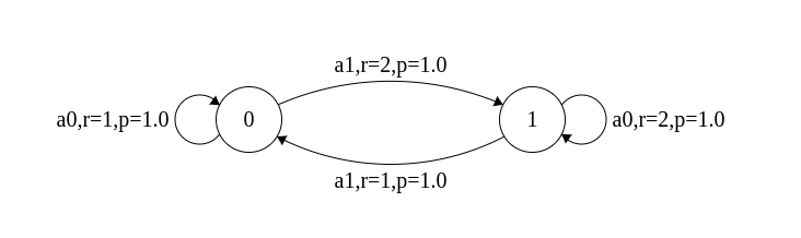
In episodic tasks, there is a terminal state: the agent's life ends as soon as it enters the terminal state. By convention, the value of the terminal state is taken as zero. Conceptually, there is no need for policies to specify actions from terminal states.

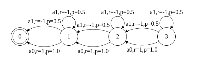
The figure below corresponds to an episodic task with 4 states, with state 0 being terminal. Take the discount factor as 0.9. From each of the states 1, 2, and 3, action a0 deterministically takes the agent left, while action a1 either carries it left or keeps it in the same state (each with probability 0.5). a0 gives positive rewards, while a1 gives negative rewards. It is not hard to see that a0 is the optimal action from each of the non-terminal states. Under the optimal policy, the value of state 1 is 1, the value of state 2 is 1 + 0.9 = 1.9, and the value of state 3 is 1 + 0.9 + 0.81 = 2.71. This MDP is available as mdpfile02.txt

Value Iteration

Value iteration is a simple, iterative algorithm, which is specified in the notes provided in class. Assume \(V^{0}\), the initial value vector, has every element as zero. Terminate when for every state \(s\), \(|V_t(s) - V_{t - 1}(s)| <= 10^{-16}\). You can assume that at this point, \(V_{t}\) is the optimal value function. An optimal policy can be obtained by taking greedy actions with respect to the optimal value function.

You will have to handle two novel aspects as a part of your implementation. First, observe that only those transitions that have non-zero probabilities are given to you in the input MDP file. In the Bellman Optimality Operator, it should suffice for you to iterate only over next states that have a non-zero probability of being reached. It would consume additional time to unnecessarily iterate over zero-probability transitions; make sure your internal data structures and code implement the efficient version.

How should you handle the end state? Fix its value to be zero, and do not update it. However, you will still use its (zero) value on the RHS of the Bellman Optimality update.

Task 1 (5 marks)

Given an MDP, your code must compute the optimal value function \(V^{\star}\) and an optimal policy \(\pi^{\star}\). Its output, written to standard output, must be in the following format.

The first \(S\) lines contain the optimal value function for each state and the action taken by an optimal policy for the corresponding state. The last line specifies the number of iterations taken by value iteration (the value of variable \(t\) in the pseudocode upon termination). In the data directory enclosed, you will find three solution files corresponding to the MDP files, which have solutions in the format above. Naturally, the number of iterations you obtain need not match the number provided in the solution, since it will depend on your implementation. The optimal policy also need not be the same, in case there are multiple optimal policies. Make sure the optimal value function matches, up to 6 decimal places.

Since your output will be checked automatically, make sure print nothing to stdout other than the \(S + 1\) lines as above in sequence. Print the action taken from the end state (if any) as -1.

Implement value iteration in any programming language of your choice (provided it can be tested on the SL2 machines), taking in an MDP file as input, and producing output in the format specified above. The first step in your code must be to read the MDP into memory; the next step to perform value iteration; and the third step to print the optimal value function, optimal policy, and number of iterations to stdout. Make sure your code produces output that matches what has been provided for the three test instances.

Create a shell script called valueiteration.sh, which will be called using the command below.

Here mdpFileName will include the full path to the MDP file; it will be the only command line argument passed. (If, say, you have implemented your algorithm in C++, the shell script must compile the C++ file and run the corresponding binary with the MDP it is passed.) The shell script must write the correct output to stdout. It is okay to use libraries and high-level templates for data structures and for operations such as finding the maximum. However, the logic used in value iteration must entirely be code that you have written.

Task 2 (5 marks)

In this task your objective is to find the shortest path from tart to end in a specified maze. The idea is to piggyback on the value iteration code you have already written for Task 1.

Your first step is to should encode the maze given as an MDP (use the same format as described above). Then you will use ./valueiteration.sh to find an optimal policy. Finally, you will extract a path from start to end based on the optimal policy. Output the path as
A0 A1 A2 . . .
where A0 A1 A2 ... is the sequence of actions taken from the start state to reach the end state along the shortest path. Each action must be one of N (north), S (south), E (east), and W (west). See, for example, solution10.txt in the Task-2 directory, for an illustrative solution.

To visualise the maze, use the following command.
python visualize.py gridfile

To visualise your solution use the following command.
python visualize.py gridfile pathfile

Create a shell script called encoder.sh that will encode the maze as an MDP and output the MDP. You can use any programming language of your choice (provided it can be tested on the SL2 machines). The script is run as follows.
./encoder.sh gridfile > mdpfile
We will then run ./valueiteration.sh mdpfile > value_and_policy_file
Create a shell script called decoder.sh that will find the shortest path between the start and end states given the file value_and_policy_file and the grid. The output should be as specified above. You can use any programming language of your choice (provided it can be tested on the SL2 machines). The script is run as follows.
./decoder.sh gridfile value_and_policy_file

Evaluation

We will run your code on the MDP and maze instances provided to you. Your code should compute the correct answer for all these instances. We will also inspect your code and run it on other test cases to make sure you have implemented your algorithms correctly. If your code fails any test instances, you will be penalised based on the nature of the mistake made.

Submission

You must submit all the files needed to run your agent, including valueiteration.sh, encoder.sh, and decoder.sh. If you have used any special libraries, mention them in a text file called libraries.txt. Place all these files in a single directory named la4-rollno (substitute rollno with your roll number; for example, la4-123456789). Tar and gzip this directory; submit la4-rollno.tar.gz. on Moodle, under Lab Assignment 4.