In this assignment, you will implement on-line TD algorithms with linear function approximation. Your testbed is an MDP that is popularly known as ``Baird's counterexample''. We stick with the version described by Sutton and Barto (1998, see Example 8.3), although the counterexample is originally from a paper by Baird (1995). You will have to experiment with two different updating schemes, and describe your results.

MDP

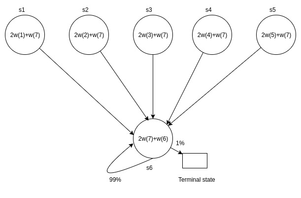
The MDP shown in the figure consists of 6 non-terminal states and 1 terminal state. It is an episodic MDP. Episodes start in one of the five upper states (picked uniformly at random), and proceed immediately to the lower state. When the agent takes (the only available) action in the lower state, it remains in the same state with probability 99%; with probability 1% it goes to the terminal state (and the episode ends). Take the discount factor γ to be 0.99. All rewards are zero rewards. By default the value of the terminal state is also taken to be zero.

Assignment

Your aim is to perform policy evaluation: that is, to estimate the value function of the policy being followed. The value of each state is to be ``approximated'' as a linear combination of features. The parameters to be learned are coefficients w(1) through w(7). The actual approximations for each state are shown in the figure: for example, V(s₂) ≈ 2 w₂ + w₇. It is easy to see that there exist several configurations of the weights that give the exact value function, which is uniformly zero. Your objective is to test two different TD variants for convergence to the zero value function, and so you will run the following two experiments. Assume that a total of N updates are performed.

1. Repeat N times: Pick a non-terminal state s in a round-robin manner, and pick next state s' according to the dynamics of the MDP: if s is among the upper states, s' is s₆; if s is s₆, then s' is s₆ with probability 99%, and the terminal state with probability 1%. Update the value function of based on a TD(0)-type update (Section 8.2, Sutton and Barto (1998)). Take the learning rate α to be a constant 0.001 (if you like, you can tune the learning rate).
2. Implement episodic TD(λ) (Section 8.2, Sutton and Barto (1998)): that is, start each episode in one of s₁ – s₅ (picked uniformly at random), and follow the dynamics of the MDP until the episode ends (each episode is likely to last about a 100 steps on account of the self-transitions in s₆). Make a TD(λ) update after each transition (with α as above). Stop the experiment after N updates have been made (N will be much larger than the average episodic length, and so you will simulate multiple episodes).

Submission

You will submit two items: (1) working code which implements the two experiments above, and (2) a report (as a single file, report.pdf) containing graphs and answers to the questions given below.

Create a directory titled [rollnumber]. Place all your source and executable files, along with the report.pdf file in this directory. The directory must contain a shell script named startmdp.sh. You are free to implement your algorithm in a programming language of your choice. startmdp.sh should take command-line arguments in the following sequence.

• Experiment number: 1 or 2
• Number of steps N
• λ
• Initial values for w(1), w(2), w(3), w(4), w(5), w(6), and w(7), respectively

Here are a couple of examples of usage.

The output of the script must be the estimated value function after each TD update. Each line must have 6 values (in sequence for states s₁ through s₆) separated by spaces. There must be a total of N lines. Make sure that your script does not output anything other than these 6N numbers.

Your code will be tested by running an experiment that calls startmdp.sh in your directory with a valid set of parameters. Before you submit, make sure you can successfully run startmdp.sh on the sl2 machines (sl2-*.cse.iitb.ac.in).

1. For experiment 1, plot a graph with the number of updates as the x axis, and the estimated value as the y axis. Set the initial weights all to 1, and take N = 1000000. Plot a separate line for each non-terminal state. What do you observe from the graph? Explain your observation.
2. For experiment 2, plot a graph with the number of updates as the X axis, and the estimated value as the y axis. Set the initial weights all to 1, and take N = 1000000. Plot a separate line for each λ in {0, 0.2, 0.4, 0.6, 0.8, 1.0}: the line must show the average of the six estimated state values. What do you observe from the graph? Explain your observation.
3. Run experiment 2 with a few different initial values for the weights (take λ = 0). Do you think the process converges to the same weights? Does it converge to the same value function?

Along with these answers, the report should also include any relevant details about your implementation of the algorithms.

Place all the data generated from your experiments, as well as report.pdf, within a directory called report, and place this directory inside your submission folder ([rollnumber]).

In summary: you must submit your [rollnumber] directory (compressed as submission.tar.gz) through Moodle. The directory must contain startmdp.sh, along with all the sources and executables. The report directory must contain all the data generated by your experiments, and a file called report.pdf

Evaluation

Your code will be tested for correctness on each experiment (2 + 2 marks); your answers in the report carry 3 marks, 2 marks, and 1 mark, in sequence.

The TAs and instructor may look at your source code and notes to corroborate the results presented in your experiments, and may also call you to a face-to-face session to explain your code.

Deadline and Rules

Your submission is due by 11.55 p.m., Friday, November 10. You are advised to finish working on your submission well in advance, keeping enough time to test it on the sl2 machines and upload to Moodle. Your submission will not be evaluated (and will be given a score of zero) if it is not received by the deadline.

You must work alone on this assignment. Do not share any code (whether yours or code you have found on the Internet) with your classmates. Do not discuss the design of your agent with anybody else.

You will not be allowed to alter your code in any way after the submission deadline. Before submission, make sure that it runs for a variety of experimental conditions on the sl2 machines. If your code requires any special libraries to run, it is your responsibility to get those libraries working on the sl2 machines (go through the CSE bug tracking system to make a request to the system administrators.)