The views that we get in the game of cricket include close-up of the players, and a variety of views that we now define:
- Pitch Views (P) bowler run-up, ball bowled, ball played.
- Ground View (G) ball tracking by camera, ball fielded and returned.
- Non-Field Views (N) Any view that is not P or G. This includes views such as the close-up of batsman, bowler, umpire, and the audience.
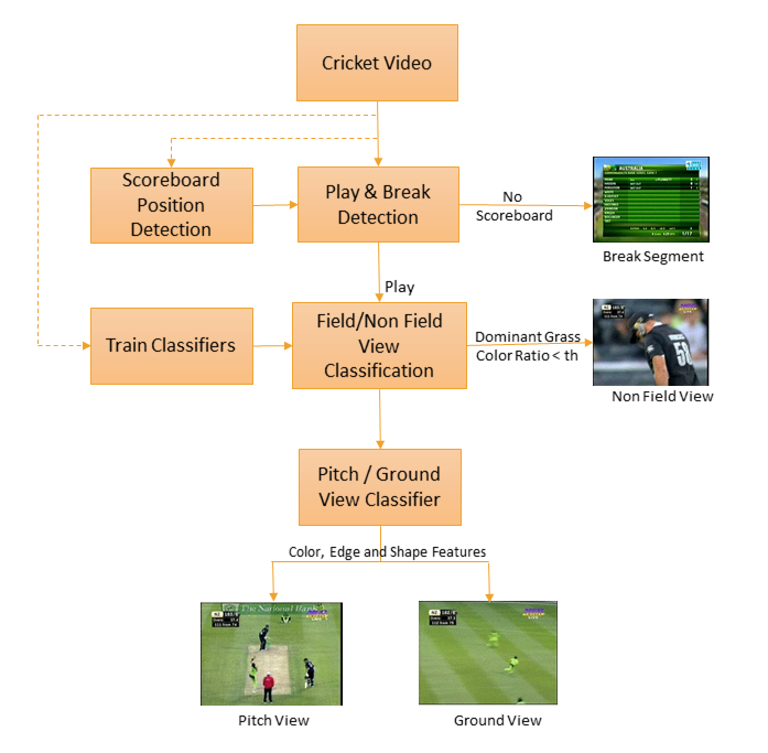
Fig. 2. Block diagram of our system
Further, it becomes useful to define Field Views (F) as the union of P and G. Using this vocabulary, we create an alphabetical sequence (see the block diagram of our system in Fig. 2.) Representative views are shown in Fig. 1. Note that our particular classification is not intended to be definitive, or universal. It may appear to be even subjective. Since our objective is not classification of views in their own right, but to get temporal segmentation, the exact clinical, or mathematical, definition of these views is unnecessary. The process of creating our sequence is Segment the video into play and break segments frames.
- Classify play segment frames into F or N
- Classify F View frames into P or G
- Smooth the resulting sequence
- Extract balls using a rule based system.
Play Time
Broadcast cricket video also contain non-play segments such as replays and advertisements. From the telecast of different matches, it is observed that for advertisements and replays, the scoreboard is not shown. Also, the location of the scoreboard is always fixed for a particular match. Hence the presence or absence of scoreboard is used to distinguish between the broadcast of match and advertisement or replay segments. A similar approach has been used in [3] to filter the replay and advertisement segments from baseball videos for event detection. In an offline stage, we take the initial 15 minute segment of videos and apply the temporal averaging approach proposed in [4] for detection and recognition of scoreboard caption for baseball videos. (In our implementation, we have seen two cases for scoreboard position: at the top left or at the bottom of the frame. The result of scoreboard position detection is shown in Fig. 3.)

Fig. 3. Scoreboard Position Detection
Extracted scoreboard and its bounding rectangle are saved. Now, for each frame of the video we crop the area specified by the bounding rectangle of the scoreboard. We compute the correlation between this cropped image and the stored scoreboard image. If the correlation is greater than a threshold T, we conclude that the frame contains scoreboard and it is classified as play segment frame; otherwise it is break segment frame.
Unfortunately, there are further complications; advertisements pop up during a cricket match and they do not cover the whole frame, but changes the score board position. Analyzing such frames, we see pop-up advertisements are relatively static as compared to the 'play' portion where there is, almost by definition, activity (that is why the advertiser wants his advertisement!). This observation is used to detect and eliminate annoying pop-up advertisements. The changed position of the 'scoreboard' is such that the boundary of the advertisement can be ascertained. The scoreboard is looked for in the quadrant where scoreboard occurs normally and based on the displacement caused due to the pop-ups, advertisement boundaries are detected. Such advertisements are removed, and the frame can now be correctly classified as play or break segments even when pop-up advertisements are present.
Field View Determination
We have used two classifiers in tandem to further process play segments. The first classifier labels the play segment frames into Field or Non-Field Views. As the name implies, the nonfield view is simply a view that is not a field view. To distinguish these views we use color information. We used the approach proposed by [4, 5] in our work. We plot the 256- bin Hue histogram for each of these views. It has been observed that the dominant peak in the case of Field View occurs only within a particular range (see Fig. 4). This interval may be different for different matches, and broadcasters, but it is quite prominent. For Non-Field Views, dominant peaks do not overlap with this interval as shown in Fig. 5.
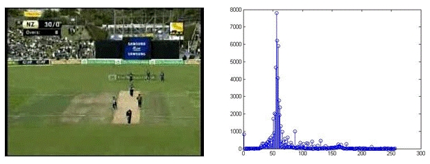
Fig. 4. Field View and its hue histogram
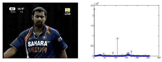
Fig. 5. Non-Field View and its hue histogram
We use this observation to compute a feature called Dominant Grass Color Ratio
where xg is the frequency of the dominant peak in a specific interval determined from training frames and M, N are rows and columns of the image [2]. We select a threshold (0.055) based on our training data. Using this threshold we classify the frames into field or non-field View. Every face detected in the current frame is then voted for a confirmation by attempting to track them in subsequent frames in the window. Confirmed faces are stored for the next step in the processing in a data matrix. Confirmed faces from each highlight i, is stored in the corresponding data matrix Di as illustrated in the Figure.
Pitch View determination
One of the two outputs of the previous classifier (i.e., Field View frames) becomes the input for the next classifier. This classifier uses a set of features described below:
- Color Histogram: It serves as an effective representation of the color content of an image if the color pattern is unique compared with the rest of the data set. The color histogram is easy to compute and effective in characterizing both the global and local distributions of colors in an image. A 128-bin Hue histogram is used in our approach.
- Edge Direction: Histogram The edges provide useful information about the structural details of the image. 4-bin edge histogram is used to represent the strength of edges in 0, π/4 , π/2 , and 3π/4 directions. Sobel operator is used to compute the edge map. Edge direction computed from edge map is then uniformly quantized to 4 bins. Edge histogram is then normalized with respect to the image size.
- Shape Features: Shape of the pitch is a prominent feature that distinguishes it with the ground view. Frames are first converted to grey images. A threshold (0.6 in our case) is applied to separate the background from pitch. Then the maximum connected area in the image is selected and properties such as Area, Orientation, Eccentricity and Centroid are computed.
- Block Histogram: The frame is divided into 3x3 blocks and 128-bin hue histogram of each block are computed.
Sequence Analysis
At this step each frame of the play segment is labeled with P, G, or N. Due to errors in classification there may be some outliers. We smooth the sequence to remove those outliers. We process the frames at an interval of 5. It has been found that each view (P, G, and N) will last for at least 20–25 frames. So, we use a sliding window of size 5 to smooth the sequence. We take the majority within this window and the center frame in this window is assigned with the label of majority view. Processed sequence is then analyzed to extract balls using the rule: A ball starts with a Pitch View and ends with a Non- Field View.
Player Detection
Once deliveries are detected, further filtering of the video is possible. For example, we consider classifying deliveries based on an a particular player, such as the Australian cricket captain Steve Smith.
We can use a standard frontal face detector to detect faces of bowlers. On the other hand, faces of batsmen are confused by the usual use of helmets. So we look for additional information in the form of connected regions (in skin color range), and square regions which have more edges. For each delivery, face detection is performed for 100 frames before and after the actual delivery. This buffer of 200 frames is assessed for recognizing faces of key players associated with the actual delivery. The usual method of dimensionality reduction, and clustering is used to prune the set. With this background, if an input image of a particular player is given, the image is mapped to the internal low dimension representation and the closest cluster is found using a kd-tree. Corresponding deliveries in which that player appears are displayed.